17  Boosting Methods

Abstract

TODO (150-200 WORDS)

Major changes expected!

This page is a work in progress and major changes will be made over time.

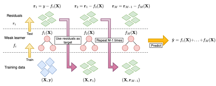
Boosting is a machine learning strategy that can be applied to any model class. Similarly to random forests, boosting is an ensemble method that creates a model from a ‘committee’ of learners. The committee is formed of weak learners that make poor predictions individually, which creates a slow learning approach (as opposed to ‘greedy’) that requires many iterations for a model to be a good fit to the data. Boosting models are similar to random forests in that both make predictions from a large committee of learners. However the two differ in how the members of the committee are correlated and in how they are combined to make a prediction. In random forests, each decision tree is grown independently and their predictions are combined by a simple mean calculation. In contrast, weak learners in a boosting model are fit sequentially with errors from one learner used to train the next, predictions are then made by a linear combination of predictions from each learner (Figure 17.1).

17.1 GBMs for Regression

One of the earliest boosting algorithms is AdaBoost (Freund and Schapire 1996), which is more generally a Forward Stagewise Additive Model (FSAM) with an exponential loss (Hastie, Tibshirani, and Friedman 2001). Today, the most widely used boosting model is the Gradient Boosting Machine (GBM) (J. H. Friedman 2001) or extensions thereof.

Figure 17.1 illustrates the process of training a GBM in a least-squares regression setting:

1. A weak learner, \(f_1\), often a decision tree of shallow depth is fit on the training data \((\mathbf{X}, \mathbf{y})\).
2. Predictions from the learner, \(f_1(\mathbf{X})\), are compared to the ground truth, \(\mathbf{y}\), and the residuals are calculated as \(\mathbf{r}_1 = f_1(\mathbf{X}) - \mathbf{y}\).
3. The next weak learner, \(f_2\), uses the previous residuals for the target prediction, \((\mathbf{X}, \mathbf{r}_1)\)
4. This is repeated to train \(M\) learners, \(f_1,...,f_M\)

Predictions are then made as \(\hat{\mathbf{y}} = f_1(\mathbf{X}) + f_2(\mathbf{X}) + ... + f_M(\mathbf{X})\).

Figure 17.1: Least squares regression Boosting algorithm where the gradient is calculated as the difference between ground truth and predictions.

This is a simplification of the general gradient boosting algorithm, where the residuals are used to train the next model. More generally, a suitable, differentiable loss function relating to the problem of interest is chosen and the negative gradient is computed by comparing the predictions in each iteration with the ground truth. Residuals can be used in the regression case as these are proportional to the negative gradient of the mean squared error.

The algorithm above is also a simplification as no hyper-parameters other than \(M\) were included for controlling the algorithm. In order to reduce overfitting, three common hyper-parameters are utilised:

Number of iterations, \(M\): The number of iterations is often claimed to be the most important hyper-parameter in GBMs and it has been demonstrated that as the number of iterations increases, so too does the model performance (with respect to a given loss on test data) up to a certain point of overfitting (Buhlmann 2006; Hastie, Tibshirani, and Friedman 2001; Schmid and Hothorn 2008a). This makes sense as the foundation of boosting rests on the idea that weak learners can slowly be combined to form a single powerful model. Finding the optimal value of \(M\) is critical as a value too small will result in poor predictions, whilst a value too large will result in model overfitting.

Subsampling proportion, \(\phi\): Sampling a fraction, \(\phi\), of the training data at each iteration can improve performance and reduce runtime (Hastie, Tibshirani, and Friedman 2001), with \(\phi = 0.5\) often used. Motivated by the success of bagging in random forests, stochastic gradient boosting (J. Friedman 1999) randomly samples the data in each iteration. It appears that subsampling performs best when also combined with shrinkage (Hastie, Tibshirani, and Friedman 2001) and as with the other hyper-parameters, selection of \(\phi\) is usually performed by nested cross-validation.

Step-size, \(\nu\): The step-size parameter is a shrinkage parameter that controls the contribution of each weak learner at each iteration. Several studies have demonstrated that GBMs perform better when shrinkage is applied and a value of \(\nu = 0.1\) is often suggested (Buhlmann and Hothorn 2007; Hastie, Tibshirani, and Friedman 2001; J. H. Friedman 2001; Lee, Chen, and Ishwaran 2019; Schmid and Hothorn 2008a). The optimal values of \(\nu\) and \(M\) depend on each other, such that smaller values of \(\nu\) require larger values of \(M\), and vice versa. This is intuitive as smaller \(\nu\) results in a slower learning algorithm and therefore more iterations are required to fit the model. Accurately selecting the \(M\) parameter is generally considered to be of more importance, and therefore a value of \(\nu\) is often chosen heuristically (e.g. the common value of \(0.1\)) and then \(M\) is tuned by cross-validation and/or early-stopping, which is the process of monitoring the model’s training performance and stopping when a set performance is reached or when performance stagnates (i.e., no improvement over a set number of rounds).

As well as these parameters, the underlying weak learner hyper-parameters are also commonly tuned. If using a decision tree, then it is usual to restrict the number of terminal nodes in the tree to be between \(4\) and \(8\), which corresponds to two or three splits in the tree. Including these hyper-parameters, the general gradient boosting machine algorithm is as follows:

1. \(g_0 \gets \text{ Initial guess}\)
2. For \(m = 1,...,M\):
3.      \(\mathcal{D}_{train}^* \gets \text{ Randomly sample } \mathcal{D}_{train}\text{ with probability } \phi\)
4.      \(r_{im} \gets -[\frac{\partial L(y_i, g_{m-1}(X_i))}{\partial g_{m-1}(X_i)}], \forall i \in \{i: X_i \in \mathcal{D}_{train}^*\}\)
5.      Fit a weak learner, \(h_m\), to \((\mathbf{X}, \mathbf{r}_m)\)
6.      \(g_m \gets g_{m-1} + \nu h_m\)
7. end For
8. return \(\hat{g}= g_M\)

Note:

1. The initial guess, \(g_0\), is often the mean of \(y\) for regression problems but can also simply be \(0\).
2. Line 4 is the calculation of the negative gradient, which is equivalent to calculating the residuals in a regression problem with the mean squared error loss.
3. Lines 5-6 differ between implementations, with some fitting multiple weak learners and selecting the one that minimizes a simple optimization problem. The version above is simplest to implement and quickest to run, whilst still providing good model performance.

Once the model is trained, predictions are made for new data, \(\mathbf{X}_{test}\) with

\[ \hat{Y}= \hat{g}(\mathbf{X}_{test}) = g_0(\mathbf{X}_{test}) + \nu \sum^M_{i=1} g_i(\mathbf{X}_{test}) \]

GBMs provide a flexible, modular algorithm, primarily comprised of a differentiable loss to minimise, \(L\), and the selection of weak learners. This chapter focuses on tree-based weak learners, though other weak learners are possible. Perhaps the most common alternatives are linear least squares (J. H. Friedman 2001) and smoothing splines (Bühlmann and Yu 2003), we will not discuss these further here as decision trees are primarily used for survival analysis, due the flexibility demonstrated in Section 15.1. See references at the end of the chapter for other weak learners. Extension to survival analysis therefore follows by considering alternative losses.

17.2 GBMs for Survival Analysis

Unlike other machine learning algorithms that historically ignored survival analysis, early GBM papers considered boosting in a survival context (Ridgeway 1999); though there appears to be a decade gap before further considerations were made in the survival setting. After that period, developments, discussed in this chapter, by Binder, Schmid, and Hothorn, adapted GBMs to a framework suitable for survival analysis.

All survival GBMs make ranking predictions and none are able to directly predict survival distributions. However, depending on the underlying model, the predictions may be indirectly composed into a survival distribution, for example algorithms that assume a proportional hazards (PH) or accelerated failure time (AFT) form. This section starts with those models with simpler underlying forms, then explores more complex alternatives.

17.2.1 PH and AFT GBMs

The negative log-likelihood of the semi-parametric PH and fully-parametric AFT models can be derived from the (partial) likelihoods presented in Section 4.1.5. Given the likelihoods measure the goodness of fit of model parameters, algorithms that use these losses use boosting to train the model coefficients, \(\boldsymbol{\beta}\), hence at each iteration in the algorithm, \(g_m(\mathbf{x}_i) = \mathbf{x}_i\boldsymbol{\beta}^{(m)}\), where \(\boldsymbol{\beta}^{(m)}\) are the updated coefficients in iteration \(m\).

The Cox partial likelihood (Cox 1972, 1975) is given by

\[ L^{PH}(\boldsymbol{\beta}) = \prod^n_{i:\delta_i=1} \frac{\exp(\eta_i)}{\sum^n_{j \in \mathcal{R}_{t_i}} \exp(\eta_j)} \]

with corresponding negative log-likelihood

\[ -l^{PH}(\boldsymbol{\beta}) = -\sum^n_{i=1} \delta_i \Big[\eta_i \ - \ \log\Big(\sum^n_{j \in \mathcal{R}_{t_i}} \exp(\eta_i)\Big)\Big] \tag{17.1}\] where \(\mathcal{R}_{t_i}\) is the set of patients at risk at time \(t_i\) and \(\eta_i = \mathbf{x}_i\boldsymbol{\beta}\).

The gradient of \(-l^{PH}\) at iteration \(m\) is then \[ r_{im} := \delta_i - \sum^n_{j=1} \delta_j \frac{\mathbb{I}(t_i \geq t_j) \exp(g_{m-1}(\mathbf{x}_i))}{\sum_{k \in \mathcal{R}_{t_j}} \exp(g_{m-1}(\mathbf{x}_k))} \tag{17.2}\] where \(g_{m-1}(\mathbf{x}_i) = \mathbf{x}_i\boldsymbol{\beta}^{(m-1)}\).

For non-PH data, boosting an AFT model can outperform boosted PH models (Schmid and Hothorn 2008b). The AFT is defined by \[ \log \mathbf{y}= \boldsymbol{\eta}+ \sigma W \] where \(W\) is a random noise variable independent of \(X\), and \(\sigma\) is a scale parameter controlling the amount of noise; again \(\boldsymbol{\eta}= \mathbf{X}\boldsymbol{\beta}\). By assuming a distribution on \(W\), a distribution is assumed for the full parametric model. The model is boosted by simultaneously estimating \(\sigma\) and \(\boldsymbol{\beta}\). Assuming a location-scale distribution with location \(g(\mathbf{x}_i)\) and scale \(\sigma\), one can derive the negative log-likelihood in the \(m\)th iteration as (Klein and Moeschberger 2003)

\[ \begin{split} -l^{AFT}_m(\boldsymbol{\beta}) = -\sum^n_{i=1} \delta_i\Big[- \log\sigma + \log f_W\Big(\frac{\log(t_i) - \hat{g}_{m-1}(\mathbf{x}_i)}{\hat{\sigma}_{m-1}}\Big)\Big] + \\ (1-\delta_i)\Big[\log S_W\Big(\frac{\log(t_i) - \hat{g}_{m-1}(\mathbf{x}_i)}{\hat{\sigma}_{m-1}}\Big)\Big] \end{split} \]

where \(\hat{g}_{m-1}, \hat{\sigma}_{m-1}\) are the location-scale parameters estimated in the previous iteration. Note this key difference to other GBM methods in which two estimates are made in each iteration step. After updating \(\hat{g}_m\), the scale parameter, \(\hat{\sigma}_m\), is updated as \[ \hat{\sigma}_m := \operatorname{argmin}_\sigma -l^{AFT}_m(\boldsymbol{\beta}) \] \(\sigma_0\) is commonly initialized as \(1\) (Schmid and Hothorn 2008b).

As well as boosting fully-parametric AFTs, one could also consider boosting semi-parametric AFTs, for example using the Gehan loss (Johnson and Long 2011) or using Buckley-James imputation (Wang and Wang 2010). However, known problems with semi-parametric AFT models and the Buckey-James procedure (Wei 1992), as well as a lack of off-shelf implementation, mean that these methods are rarely used in practice.

17.2.2 Discrimination Boosting

Instead of optimising models based on a given model form, one could instead estimate \(\hat{\eta}\) by optimizing a concordance index, such as Uno’s or Harrell’s C (Y. Chen et al. 2013; Mayr and Schmid 2014). Consider Uno’s C (Section 8.1): \[ C_U(\hat{g}, \mathcal{D}_{train}) = \frac{\sum_{i \neq j}\delta_i\{\hat{G}_{KM}(t_i)\}^{-2}\mathbb{I}(t_i < t_j)\mathbb{I}(\hat{g}(\mathbf{x}_i) >\hat{g}(\mathbf{x}_j))}{\sum_{i \neq j}\delta_i\{\hat{G}_{KM}(t_i)\}^{-2}\mathbb{I}(t_i < t_j)} \]

The GBM algorithm requires that the chosen loss, here \(C_U\), be differentiable with respect to \(\hat{g}(X)\), which is not the case here due to the indicator term, \(\mathbb{I}(\hat{g}(X_i) > \hat{g}(X_j))\), however this term can be replaced with a sigmoid function to create a differentiable loss (Ma and Huang 2006)

\[ K(u|\omega) = \frac{1}{1 + \exp(-u/\omega)} \]

where \(\omega\) is a tunable hyper-parameter controlling the smoothness of the approximation. The measure to optimise is then,

\[ C_{USmooth}(\boldsymbol{\beta}|\omega) = \sum_{i \neq j} \frac{k_{ij}}{1 + \exp\big[(\hat{g}(X_j) - \hat{g}(X_i))/\omega)\big]} \tag{17.3}\]

with

\[ k_{ij} = \frac{\Delta_i (\hat{G}_{KM}(T_i))^{-2}\mathbb{I}(T_i < T_j)}{\sum_{i \neq j} \Delta_i(\hat{G}_{KM}(T_i))^{-2}\mathbb{I}(T_i < T_j)} \]

The negative gradient at iteration \(m\) for observation \(i\) is then calculated as,

\[ r_{im} := - \sum^n_{j = 1} k_{ij} \frac{-\exp(\frac{\hat{g}_{m-1}(\mathbf{x}_j) - \hat{g}_{m-1}(\mathbf{x}_i)}{\omega})}{\omega(1 + \exp(\frac{\hat{g}_{m-1}(\mathbf{x}_j) - \hat{g}_{m-1}(\mathbf{x}_i)}{\omega}))} \tag{17.4}\]

The GBM algorithm is then followed as normal with the above loss and gradient. This algorithm may be more insensitive to overfitting than others (Mayr, Hofner, and Schmid 2016), however stability selection (Meinshausen and Bühlmann 2010), which is implemented in off-shelf software packages (Hothorn et al. 2020), can be considered for variable selection.

17.2.3 CoxBoost

Finally, ‘CoxBoost’ is an alternative method to boost Cox models and has been demonstrated to perform well in experiments. This algorithm boosts the Cox PH by optimising the penalized partial-log likelihood; additionally the algorithm allows for mandatory (or ‘forced’) covariates (Binder and Schumacher 2008). In medical domains the inclusion of mandatory covariates may be essential, either for model interpretability, or due to prior expert knowledge. CoxBoost deviates from the algorithm presented above by instead using an offset-based approach for generalized linear models (Tutz and Binder 2007).

Let \(\mathcal{I}= \{1,...,p\}\) be the indices of the covariates, let \(\mathcal{I}_{mand}\) be the indices of the mandatory covariates that must be included in all iterations, and let \(\mathcal{I}_{opt} = \mathcal{I}\setminus \mathcal{I}_{mand}\) be the indices of the optional covariates that may be included in any iteration. In the \(m\)th iteration, the algorithm fits a weak learner on all mandatory covariates and one optional covariate: \[ \mathcal{I}_m = \mathcal{I}_{mand} \cup \{x | x \in \mathcal{I}_{opt}\} \]

In addition, a penalty matrix \(\mathbf{P} \in \mathbb{R}^{p \times p}\) is considered such that \(P_{ii} > 0\) implies that covariate \(i\) is penalized and \(P_{ii} = 0\) means no penalization. In practice, this is usually a diagonal matrix (Binder and Schumacher 2008) and by setting \(P_{ii} = 0, i \in I_{mand}\) and \(P_{ii} > 0, i \not\in I_{mand}\), only optional (non-mandatory) covariates are penalized. The penalty matrix can be allowed to vary with each iteration, which allows for a highly flexible approach, however in implementation a simpler approach is to either select a single penalty to be applied in each iteration step or to have a single penalty matrix (Binder 2013).

At the \(m\)th iteration and the \(k\)th set of indices to consider (\(k = 1,...,p\)), the loss to optimize is the penalized partial-log likelihood given by \[ \begin{split} &l_{pen}(\gamma_{mk}) = \sum^n_{i=1} \delta_i \Big[\eta_{i,m-1} + \mathbf{x}_{i,\mathcal{I}_{mk}}\gamma^\intercal_{mk}\Big] - \\ &\quad\delta_i\log\Big(\sum^n_{j = 1} \mathbb{I}(t_j \leq t_i) \exp(\eta_{i,{m-1}} + \mathbf{x}_{i, \mathcal{I}_{mk}}\gamma^\intercal_{mk}\Big) - \lambda\gamma_{mk}\mathbf{P}_{mk}\gamma^\intercal_{mk} \end{split} \]

where \(\eta_{i,m} = \mathbf{x}_i\beta_m\), \(\gamma_{mk}\) are the coefficients corresponding to the covariates in \(\mathcal{I}_{mk}\) which is the possible set of candidates for a subset of total candidates \(k = 1,...,p\); \(\mathbf{P}_{mk}\) is the penalty matrix; and \(\lambda\) is a penalty hyper-parameter to be tuned or selected.

In each iteration, all potential candidate sets (the union of mandatory covariates and one other covariate) are updated by \[ \hat{\gamma}_{mk} = \mathbf{I}^{-1}_{pen}(\hat{\gamma}_{(m-1)k})U(\hat{\gamma}_{(m-1)k}) \] where \(U(\gamma) = \partial l / \partial \gamma (\gamma)\) and \(\mathbf{I}^{-1}_{pen} = \partial^2 l/\partial\gamma\partial\gamma^T (\gamma + \lambda\mathbf{P}_{(m-1)k})\) are the first and second derivatives of the unpenalized partial-log-likelihood. The optimal set is then found as \[ k^* := \operatorname{argmax}_k l_{pen}(\hat{\gamma}_{mk}) \] and the estimated coefficients are updated with \[ \hat{\beta}_m = \hat{\beta}_{m-1} + \hat{\gamma}_{mk^*}, \quad k^* \in \mathcal{I}_{mk} \]

This deviates from the standard GBM algorithm by directly optimizing \(l_{pen}\) and not its gradient, additionally model coefficients are iteratively updated instead of a more general model form.

17.3 Conclusion

Key takeaways

• GBMs are a highly flexible and powerful machine learning tool. They have proven particularly useful in survival analysis as minimal adjustments are required to make use of off-shelf software.
• The flexibility of the algorithm allows all the models above to be implemented in relatively few open-source packages.
• There is evidence that boosting models can outperform the Cox PH even in low-dimensional settings (Schmid and Hothorn 2008b), which is not not something all ML models can claim.

Limitations

• Boosting, especially with tree learners, is viewed as a black-box model that is increasingly difficult to interpret as the number of iterations increase. However, there are several methods for increasing interpretability, such as variable importance and SHAPs (Lundberg and Lee 2017).
• Boosting often relies on intensive computing power, however, dedicated packages such as \(\textbf{xgboost}\) (T. Chen et al. 2020), exist to push CPU/GPUs to their limits in order to optimise predictive performance.

Further reading

• Bühlmann and Yu (2003); Hothorn et al. (2020); Wang and Wang (2010) for more general information and background on componentwise GBMs
• J. H. Friedman (2001); Wang and Wang (2010) for linear least squares weak learners
• Bühlmann and Yu (2003); J. H. Friedman (2001) for decision tree weak learners
• Ridgeway (1999) for early research into GBMs for survival analysis
• Johnson and Long (2011) and Wang and Wang (2010) for semi-parametric AFT boosting

Binder, Harald. 2013. “CoxBoost: Cox models by likelihood based boosting for a single survival endpoint or competing risks.” CRAN.

Binder, Harald, and Martin Schumacher. 2008. “Allowing for mandatory covariates in boosting estimation of sparse high-dimensional survival models.” BMC Bioinformatics 9 (1): 14. https://doi.org/10.1186/1471-2105-9-14.

Buhlmann, Peter. 2006. “Boosting for high-dimensional linear models.” Ann. Statist. 34 (2): 559–83. https://doi.org/10.1214/009053606000000092.

Buhlmann, Peter, and Torsten Hothorn. 2007. “Boosting Algorithms: Regularization, Prediction and Model Fitting.” Statist. Sci. 22 (4): 477–505. https://doi.org/10.1214/07-STS242.

Bühlmann, Peter, and Bin Yu. 2003. “Boosting With the L2 Loss.” Journal of the American Statistical Association 98 (462): 324–39. https://doi.org/10.1198/016214503000125.

Chen, Tianqi, Tong He, Michael Benesty, Vadim Khotilovich, Yuan Tang, Hyunsu Cho, Kailong Chen, et al. 2020. “xgboost: Extreme Gradient Boosting.” CRAN. https://cran.r-project.org/package=xgboost.

Chen, Yifei, Zhenyu Jia, Dan Mercola, and Xiaohui Xie. 2013. “A Gradient Boosting Algorithm for Survival Analysis via Direct Optimization of Concordance Index.” Edited by Lev Klebanov. Computational and Mathematical Methods in Medicine 2013: 873595. https://doi.org/10.1155/2013/873595.

Cox, D. R. 1972. “Regression Models and Life-Tables.” Journal of the Royal Statistical Society: Series B (Statistical Methodology) 34 (2): 187–220.

———. 1975. “Partial Likelihood.” Biometrika 62 (2): 269–76. https://doi.org/10.1080/03610910701884021.

Freund, Yoav, and Robert E Schapire. 1996. “Experiments with a new boosting algorithm.” In. Citeseer.

Friedman, Jerome. 1999. “Stochastic Gradient Boosting.” Computational Statistics & Data Analysis 38 (March): 367–78. https://doi.org/10.1016/S0167-9473(01)00065-2.

Friedman, Jerome H. 2001. “Greedy Function Approximation: A Gradient Boosting Machine.” The Annals of Statistics 29 (5): 1189–1232. http://www.jstor.org/stable/2699986.

Hastie, Trevor, Robert Tibshirani, and Jerome Friedman. 2001. The Elements of Statistical Learning. Springer New York Inc.

Hothorn, Torsten, Peter Buehlmann, Thomas Kneib, Matthias Schmid, and Benjamin Hofner. 2020. “mboost: Model-Based Boosting.” CRAN. https://cran.r-project.org/package=mboost.

Johnson, Brent A, and Qi Long. 2011. “Survival ensembles by the sum of pairwise differences with application to lung cancer microarray studies.” Ann. Appl. Stat. 5 (2A): 1081–101. https://doi.org/10.1214/10-AOAS426.

Klein, John P, and Melvin L Moeschberger. 2003. Survival analysis: techniques for censored and truncated data. 2nd ed. Springer Science & Business Media.

Lee, Donald K K, Ningyuan Chen, and Hemant Ishwaran. 2019. “Boosted nonparametric hazards with time-dependent covariates.” https://arxiv.org/abs/arXiv:1701.07926v6.

Lundberg, Scott M, and Su-In Lee. 2017. “A Unified Approach to Interpreting Model Predictions.” Advances in Neural Information Processing Systems 30.

Ma, Shuangge, and Jian Huang. 2006. “Regularized ROC method for disease classification and biomarker selection with microarray data.” Bioinformatics (Oxford, England) 21 (January): 4356–62. https://doi.org/10.1093/bioinformatics/bti724.

Mayr, Andreas, Benjamin Hofner, and Matthias Schmid. 2016. “Boosting the discriminatory power of sparse survival models via optimization of the concordance index and stability selection.” BMC Bioinformatics 17 (1): 288. https://doi.org/10.1186/s12859-016-1149-8.

Mayr, Andreas, and Matthias Schmid. 2014. “Boosting the concordance index for survival data–a unified framework to derive and evaluate biomarker combinations.” PloS One 9 (1): e84483–83. https://doi.org/10.1371/journal.pone.0084483.

Meinshausen, Nicolai, and Peter Bühlmann. 2010. “Stability selection.” Journal of the Royal Statistical Society: Series B (Statistical Methodology) 72 (4): 417–73. https://doi.org/10.1111/j.1467-9868.2010.00740.x.

Ridgeway, Greg. 1999. “The state of boosting.” Computing Science and Statistics 31: 172—–181.

Schmid, Matthias, and Torsten Hothorn. 2008a. “Boosting additive models using component-wise P-splines.” Computational Statistics & Data Analysis 53 (2): 298–311.

———. 2008b. “Flexible boosting of accelerated failure time models.” BMC Bioinformatics 9 (February): 269. https://doi.org/10.1186/1471-2105-9-269.

Tutz, Gerhard, and Harald Binder. 2007. “Boosting Ridge Regression.” Computational Statistics & Data Analysis 51 (February): 6044–59. https://doi.org/10.1016/j.csda.2006.11.041.

Wang, Zhu, and C Y Wang. 2010. “Buckley-James Boosting for Survival Analysis with High-Dimensional Biomarker Data.” Statistical Applications in Genetics and Molecular Biology 9 (1). https://doi.org/https://doi.org/10.2202/1544-6115.1550.

Wei, L J. 1992. “The Accelerated Failure Time Model: A Useful Alternative to the Cox Regression Model in Survival Analysis.” Statistics in Medicine 11: 1871–79.