1 Introduction
This page is a work in progress and major changes will be made over time.
There are many books dedicated to regression and classification as machine learning problems but tthe ‘bibles’ of machine learning focus almost entirely on regression and classification (Bishop (2006); Hastie et al. (2001); James et al. (2013)). There are also excellent books dedicated to survival analysis, such as Collett (2014) and Kalbfleisch and Prentice (1973), but without the inclusion of machine learning models. Survival analysis has important applications to fields that directly impact day-to-day life, including healthcare, finance, and engineering. Using regression and classification models to solve problems based on survival datasets can lead to biased results, which in turn may have negative consequences. This book is intended to bridge the gap between survival analysis and machine learning to increase accessibility and to demystify the combined field of ‘machine learning survival analysis’.
1.1 Defining Machine Learning Survival Analysis
The purpose of this book is to formalise the use of machine learning in survival analysis, which we refer to as ‘machine learning survival analysis’. This chapter highlights the importance of survival analysis and what makes predictions in a survival setting (‘survival predictions’) stand out from other areas such as regression and classification. We begin with some examples and then introduce the most important concepts that make machine learning survival analysis unique.
1.1.1 Waiting for a bus
It is likely that you are making or using some form of survival predictions daily. For example, estimating when a bus will arrive at your stop after it leaves the previous one, is a survival prediction. On first glance, many would call this a regression problem, as regression is tasked with making continuous predictions. However, unless you are reading this from a country that has a perfect public transport system, then it is likely you are not making this prediction based simply on all previous bus arrival times, but also with the knowledge that your bus might break down before it reaches you. In survival analysis, we would refer to the act of a bus breaking down and not reaching its destination as a ‘censoring event’. An observation (in this case a bus) is censored when the event of interest (in this case, arriving at your bus stop) does not occur (in this case due to breakdown), this is illustrated in ?fig-bus. Survival analysis is unique as observations that are censored are still considered to be valuable data points to train a model on. Instead of dismissing these broken down buses, models that make survival predictions (‘survival models’) instead use all data up until the point of censoring. In other words, whilst your bus did not arrive, you do at least know that it had travelled two minutes (the ‘censoring time’) from its previous stop before you received an alert that it broke down, which is valuable information.
1.1.2 Allocating resources
The previous example covered a common use case of survival analysis, which is estimating survival times, i.e., the time at which an event of interest will occur. In practice, survival models usually estimate the survival time distribution which predicts the probability of the event over a period of time, this is more informative than just predicting a single time as the model can also attribute uncertainty to that prediction. Another common survival problem is to rank observations (often patients) or separate them into risk groups, usually for allocating scarce resources. As another example that occurs daily, take the process of triaging patients in an emergency department. A patient presents with a set of symptoms, and is then triaged, which means their symptoms are assessed and used to determine how urgently they need to receive help (or if they can be dismissed from hospital). Triaging patients is once again a survival prediction. In this case, the event of interest is an increase in severity from initial symptoms to a more serious display of illness. Reasons for censoring might include the patient leaving the hospital. In this example, the survival prediction is to estimate the risk of the event occurring relative to other patients, i.e., when a new patient is triaged, how do their symptoms compare to patients who have already been through the triage process? Are they at a higher risk and should therefore be seen by a clinician sooner? Or can they afford to wait longer than those who have already been waiting a long time?
1.1.3 ‘Survival’ analysis
While the term survival analysis does highlight the closely related nature of the field with medical statistics and in particular predicting survival times (i.e., the time until death), this is certainly not the only application of the field (as we have already seen in the bus example). In engineering, the field is often referred to as ‘reliability analysis’, as a common task is predicting the reliability of a component in a machine, for example predicting when an engine in a plane needs to be replaced. In economics, the term ‘duration analysis’ is often found, and in other areas ‘failure-time analysis’ may also be used. This book uses ‘survival analysis’ throughout as this appears to be the most common term, however the term is used in this book to specifically refer to the case when the event of interest can occur exactly once (e.g., death). In Chapter 3, ‘event history analysis’ is defined, which is a generalisation of survival analysis to the case when one or more events can occur multiple times.
One of our key aims in this book is to highlight the ubiquitous nature of survival analysis and to encourage more machine learning practitioners to use survival analysis when appropriate. Machine learning practitioners are likely familiar with regression and classification, which are the subjects of popular machine learning books (some listed above) however there will be cases when survival analysis should be used instead. The previous bus example gives one such case, where regression may appear sensible on the surface however this would not succeed in handling censored data. Another common example where survival analysis should be used but is not is to make ‘T-year’ probability predictions. These predictions are commonly found when discussing severe illnesses, for example statements such as “the five-year survival rate of cancer is p%.” On the surface this may seem like a probabilistic classification problem, but once again modelling in this way would ignore censoring, for example due to some patients being lost to follow-up. Understanding censoring in all its many forms, is the first step to identifying a survival analysis problem, the second is knowing what to predict.
1.1.4 Machine learning survival analysis
Machine learning is the field of Statistics primarily concerned with building models to either predict outputs from inputs or to learn relationships from data (Hastie et al. 2001). This book is limited to the former case, or more specifically supervised learning, as this is the field in which the vast majority of survival problems live.
Defining if a model is ‘machine learning’ is surprisingly difficult, with terms such as ‘iterative’ and ‘loss optimization’ being frequently used in often clunky definitions. This book defines machine learning models as those that:
- Require intensive model fitting procedures such as recursion or iteration;
- Are flexible in that they have hyper-parameters that can be tuned (Chapter 2);
- Trained using some form of loss optimization;
- Are ‘black boxes’ without simple closed-form expressions that can be easily interpreted;
- Aim to minimize the difference between predictions and ground truth whilst placing minimal assumptions on the underlying data form.
However, there are other models, which one might think of as a ‘traditional statistical’ models (?sec-classical), that can also be used for machine learning. These ‘traditional’ models are low-complexity models that are either non-parametric or have a simple closed-form expression with parameters that can be fit with maximum likelihood estimation (or an analogous method). Whilst these traditional models are usually fast to train and are highly interpretable, they can be inflexible and may make unreasonable assumptions as they assume underlying probability distributions to model data. Augmenting these models with certain methods, leads to powerful models that can also be considered ‘machine learning’ tools; hence their inclusion in this book.
Relative to other areas of supervised learning, development in survival analysis has been slow, as will be seen when discussing models in Part III. Despite this, development of models has converged on three primary tasks of interest, or ‘survival problems’, which are defined by the type of prediction the model makes. The formal definition of a machine learning survival analysis task is provided in Chapter 2, but informally one is encountering a survival problem if training a model on data where censoring is present in order to predict one of (Chapter 5):
- A ‘relative risk’: The risk of an event taking place.
- A ‘survival time’: The time at which the event will take place.
- A ‘survival distribution’: The probability distribution of the event times, i.e., the probability of the event occurring over time.
This presents a key difference between survival analysis and other machine learning areas. There are three separate objects that can be predicted, and not all models can predict each one. Moreover, each prediction type serves a different purpose and you may require deploying multiple models to serve each one. As an example, an engineer is unlikely to care the exact time at which a plane engine fails, but they might greatly value knowing when the probability of failure increases above 50% – a survival distribution prediction. Returning to the triage example, a physician cannot process a survival distribution prediction to make urgent decisions, but they could assign limited resources if it is clear that one patient is at far greater risk than another – a relative risk prediction.
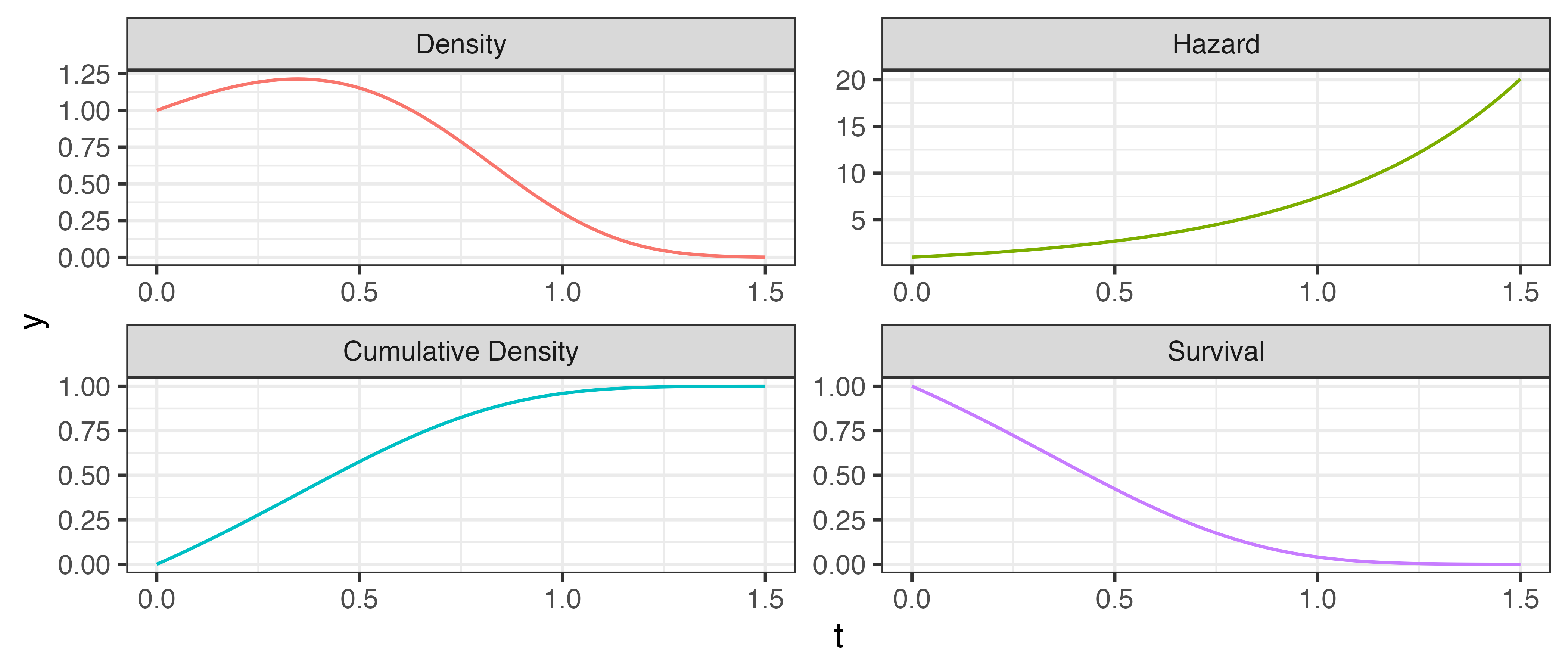
Another important difference that separates survival analysis from other statistical settings, is the focus on less common forms of distribution defining functions. A distribution defining function is a function that uniquely defines a probability distribution, most commonly the probability density function (pdf) and cumulative distribution function (cdf). In the context of survival analysis, the pdf at time \(t\) is the likelihood of an event taking place at \(t\), independently of any past knowledge, and the cdf is the probability that the event has already taken place at \(t\), which is the opposite of the usual survival prediction of interest. Hence, survival analysis predictions usually focus on predicting the survival function, which is simply one minus the cdf, and the hazard function, which is the likelihood of the event occurring at \(t\) given that the observation has survived to at least time \(t\).
These functions are formally defined in Chapter 3 and are visualized in Figure 1.1 assuming a Gompertz distribution, which is often chosen to model adult lifespans. The figure demonstrates the utility of the survival and hazard functions for survival analysis. The survival function (bottom right) is a decreasing function from one to zero, at a given time point, \(t\), this is interpreted as the probability of surviving until time point, \(t\), or more generally the probability that the event of interest has not yet occurred. The hazard function (top right), starts at zero and is not upper-bounded at one as it is a conditional probability. Even though the pdf peaks just before 0.5, the hazard function continues to increase as it is conditioned on not having experienced the event, hence the risk of event just continues to increase.
Instead of duplicating content from machine learning or survival analysis books, this book primarily focuses on defining the suitability of different methods and models depending on the availability data. For example, when might you consider a neural network instead of a Cox Proportional Hazards model? When might you use a random forest instead of a support vector machine? Is a discrimination-booted gradient boosting machine more appropriate than other objectives? Can you even use a machine learning model if you have left-censored multi-state data (we will define these terms later)?
From fitting a model to evaluating its predictions, knowing the different prediction types is vital to interpretation of results, these will be formalised in Chapter 3.
1.2 Censoring and Truncation
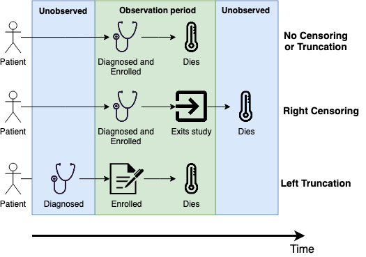
As already discussed, censoring is the defining feature of survival analysis. As well censoring, some survival problems may also deal with ‘truncation’, which can be thought of as a stricter form of censoring. In general terms, truncation is the process of fully excluding data whereas censoring is the process of partially excluding data. In survival analysis, data is measured over time and censoring or truncation apply to the survival time outcome. The precise definitions of different types of censoring and truncation are provided in Chapter 3, for now we just provide a non-technical summary of the most common form of both to highlight how prominent they are.
The most common form of censoring is right-censoring (Figure 1.2, middle), this occurs when the true survival time is ‘to the right of’, i.e., larger than (if you imagine a number line), the observed censoring time. The examples above are all forms of right-censoring. A canonical example of right-censoring is as follows: if a medical study lasts five years and patients are censored if they are alive at the end of the study, then all patients alive at five years are right-censored as their true survival time must be greater than five years.
In contrast, the most common form of truncation is left-truncation, which can occur in a few different situations and results in data before the truncation time either being partially or fully removed (Figure 1.2, bottom). The examples below look at partial left-truncation, complete truncation, and using partial truncation to fix biases.
Example 1: Partial left-truncation Say a study begins in 2024 to predict the time until death for a patient diagnosed with tuberculosis (TB) treated with a novel treatment. The study consists of many individuals, however some of these already had TB before 2024. Left-truncation would occur if the study excludes data about the individuals who had TB before 2024, i.e., treated them as if they were diagnosed with TB on entry to the study - this is partial left-truncation. Excluding this data would bias the results, especially if the novel treatment is most effective for people in the early-stages of the disease. One common way to account for this bias would be to record the initial date of diagnosis and the date the treatment began.
Example 2: Complete left-truncation Consider researchers exploring if survival models can be used to more accurately predict the exact day a pregnant person will give birth, with abortion and miscarriage treated as competing risks. Unfortunately, there will be cases of miscarriage occurring before a person finds out they are pregnant, which means data about their pregnancy will never be collected. The first, more obvious, consequence of this omission is that the true number of miscarriages will be underestimated. The second consequence is that the time until miscarriage outcome will be overestimated, as earlier miscarriages are not recorded so the outcome time is skewed towards later ones. To demonstrate why this is problematic, if someone discovers they are pregnant early and this new model is used to predict the outcome of their pregnancy, then even if it correctly predicts they have a miscarriage, it is likely to predict this happens later than it actually does, which could have an effect on any potential treatment (physical and/or mental) that may need to be allocated. The bias in this example is particularly hard to address as the data is completely truncated - the subjects are omitted without the researchers being aware of them.
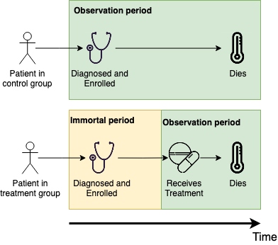
Example 3: Immortal time bias Immortal time bias occurs when an observation in the data is guaranteed to survive a period of time (hence being ‘immortal’ in that time) by virtue of the study design. For example, say a randomised controlled trial is conducted to test if a novel chemotherapy treatment improves survival rates from a given cancer. The trial is split into two arms, one for existing treatments and one for the novel treatment, and a patient is eligible for the novel treatment only if they have been living with cancer for two years and no other treatment has been shown to work. Finally, patients are enrolled into the study from the date of diagnosis. This dataset now includes immortal time bias as patients can only be in the novel treatment arm if they have already survived two years, whereas patients in the other arm have no such restriction. Hence, even if the novel treatment has no benefit, patients in the novel arm are guaranteed to have a better survival outcome (from diagnosis) as they would not have been included if they died before two years, whereas patients may die (even if by chance) in the control arm before this time (Figure 1.3). To control for this bias, one could improve the study design by considering the time to death given two years of surviving and therefore partially left-truncating data before this time. Or, one could determine eligibility at the time of diagnosis by randomly assigning patients to each group but only starting the novel treatment at two years. Detecting immortal time bias is hugely important, especially in randomised controlled trials to ensure novel treatments are not oversold.
Censoring is a mechanism applied at the data collection stage in order to yield more useful results by recording as much data as possible. Truncation is due to the study design and may either create or remove biases in data collection/curation. The first Part of this book will continue to demystify the concepts of censoring, truncation, and prediction types.
1.3 Start to finish
1.4 Reproducibility
This book includes simulations and figures generated in \(\textsf{R}\), the code for any figures or experiments in this book are freely available at https://github.com/mlsa-book/MLSA under an MIT license and all content on this website is available under CC BY 4.0.