8 Scoring Rules
This page is a work in progress and minor changes will be made over time.
Scoring rules evaluate probabilistic predictions and (attempt to) measure the overall predictive ability of a model in terms of both calibration and discrimination (Gneiting and Raftery 2007; Murphy 1973). In contrast to calibration measures, which assess the average performance across all observations on a population level, scoring rules evaluate the sample mean of individual predictions across all observations in a test set. As well as being able to provide information at an individual level, scoring rules are also popular as probabilistic forecasts are widely recognized to be superior to deterministic predictions for capturing uncertainty in predictions (Dawid 1984; Dawid 1986). Formalization and development of scoring rules has primarily been due to Dawid (Dawid 1984; Dawid 1986; Dawid and Musio 2014) and Gneiting and Raftery (Gneiting and Raftery 2007); though the earliest measures promoting “rational” and “honest” decision making date back to the 1950s (Brier 1950; Good 1952). Few scoring rules have been proposed in survival analysis, although the past few years have seen an increase in popularity in these measures. Before delving into these measures, we will first describe scoring rules in the simpler classification setting.
Scoring rules are pointwise losses, which means a loss is calculated for all observations and the sample mean is taken as the final score. To simplify notation, we only discuss scoring rules in the context of a single observation, where \(L_i(\hat{S}_i, t_i, \delta_i)\) would be the loss calculated for some observation \(i\) where \(\hat{S}_i\) is the predicted survival function (from which other distribution functions can be derived), and \((t_i, \delta_i)\) is the observed survival outcome.
8.1 Classification Losses
In the simplest terms, a scoring rule compares a probabilistic prediction to an observed outcome and assigns them a score. Formally, a loss function is written as
\[ L: \mathcal{P}\times \mathcal{Y}\mapsto \bar{\mathbb{R}}, \]
where \(p \in \mathcal{P}\) is a (predicted) probability distribution over the outcome space \(\mathcal{Y}\) and \(Y\) is a random variable representing the ground truth. In classification tasks, \(\mathcal{Y}\subseteq \mathbb{N}_0\).
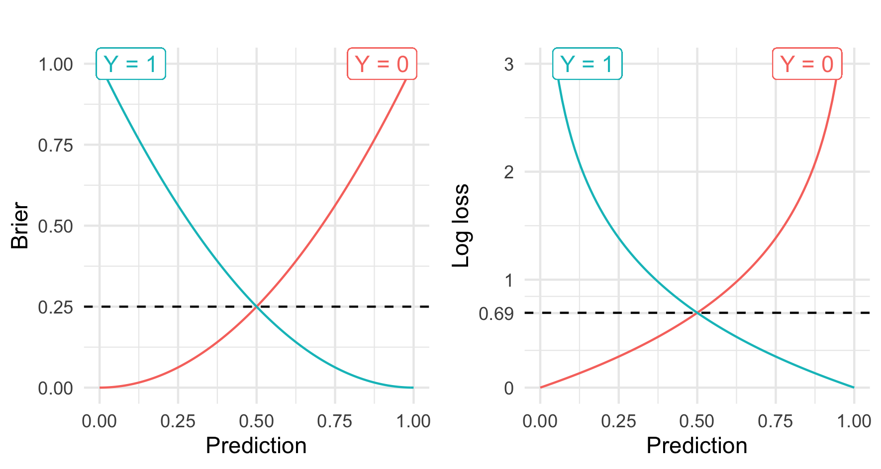
As an example, take the Brier score (Brier 1950) defined by: \[ L_{Brier}(\hat{p}_i, y_i) = (y_i - \hat{p}_i(y_i))^2 \]
For a binary classification problem, \(\hat{p}_i\) is a predicted probability mass function such that \(\hat{p}_i(x) \in [0,1]\) and \(y_i \in \{0,1\}\) is the ground truth. This scoring rule compares the ground truth to the predicted probability by testing if the difference between the observed event and the truth is minimized. This is intuitive: if the event occurs and \(y_i = 1\), then \(\hat{p}_i(y_i)\) should be as close to one as possible to minimize the loss. On the other hand, if \(y_i = 0\) then the better prediction would be \(\hat{p}_i(y_i) = 0\).
This demonstrates an important property of the scoring rule, properness. A loss is proper if it is minimized by the correct prediction. In contrast, the loss \(L_{improper}(\hat{p}_i, y_i) = 1 - L_{Brier}(\hat{p}_i, y_i)\) is still a scoring rule as it compares the ground truth to the prediction probability distribution, but it is clearly improper as the perfect prediction (\(\hat{p}_i(y_i) = y_i\)) would result in a score of \(1\) whereas the worst prediction would result in a score of \(0\). Proper losses provide a method of model comparison as, by definition, predictions closest to the true distribution will result in lower expected losses.
Another important property is strict properness. A loss is strictly proper if the loss is uniquely minimized by the ‘correct’ prediction. For example, the Brier score is minimized by only one value, which is the optimal prediction Figure 8.1. Strictly proper losses are particularly important for automated model optimization, as minimization of the loss will result in the ‘optimum score estimator based on the scoring rule’ (Gneiting and Raftery 2007).
Mathematically, a classification loss \(L: \mathcal{P}\times \mathcal{Y}\rightarrow \bar{\mathbb{R}}\) is proper if for any distributions \(p_Y,p\) in \(\mathcal{P}\) and for any random variables \(Y \sim p_Y\) (with observations \(y_i\)), it holds that \(\mathbb{E}[L(p_Y, Y)] \leq \mathbb{E}[L(p, Y)]\). The loss is strictly proper if, in addition, \(p = p_Y\) uniquely minimizes the loss.
As well as the Brier score, which was defined above, another widely used loss is the log loss (Good 1952), defined by
\[ L_{logloss}(\hat{p}_i, y_i) = -\log \hat{p}_i(y_i) \tag{8.1}\]
where again \(y_i \in \{0,1\}\) is the ground truth and \(\hat{p}_i\) is a predicted probability distribution.
These losses are visualized in Figure 8.1, which highlights that both losses are strictly proper (Dawid and Musio 2014) as they are minimized when the true prediction is made, and converge to the minimum as predictions are increasingly improved. It can also be seen from the scale of the plots that the log-loss penalizes wrong predictions more strongly than the Brier score, which may be beneficial or not depending on the given use-case.
8.2 Survival Losses
Analogously to classification losses, one can define a survival loss as
\[ L_S: \mathcal{P}\times \mathbb{R}_{>0}\times \{0,1\}\rightarrow \bar{\mathbb{R}}, \]
where now \(\mathcal{P}\) denotes a set of probability distributions over \(\mathbb{R}_{>0}\). \(L_S\) is proper if for any distributions \(p_Y, p\) in \(\mathcal{P}\), and for any random variables \(Y \sim p_Y\), and \(C\) taking values in \(\mathbb{R}_{>0}\); with \(T := \min(Y,C)\) and \(\Delta := \mathbb{I}(T=Y)\); it holds that, \(\mathbb{E}[L_S(p_Y, T, \Delta)] \leq \mathbb{E}[L_S(p, T, \Delta)]\). The loss is strictly proper if, in addition, \(p = p_Y\) uniquely minimizes the loss. A survival loss is referred to as outcome-independent (strictly) proper if it is only (strictly) proper when \(C\) and \(Y\) are independent.
With these definitions, the rest of this chapter lists common scoring rules in survival analysis and discusses some of their properties. As with other chapters, this list is likely not exhaustive but will cover commonly used losses. The losses are grouped into squared losses, absolute losses, and logarithmic losses, which respectively estimate the mean squared error, mean absolute error, and log loss in uncensored settings.
8.2.1 Squared Losses
The Integrated Survival Brier Score (ISBS) was introduced by Graf (Graf and Schumacher 1995; Graf et al. 1999) as an analogue to the integrated Brier score in regression. It is likely the most commonly used scoring rule in survival analysis, possibly due to its intuitive interpretation.
The loss is defined by
\[ \begin{split} L_{ISBS}(\tau^*, \hat{S}_i, t_i, \delta_i|\hat{G}_{KM}) = \int^{\tau^*}_0 \frac{\hat{S}_i^2(\tau) \mathbb{I}(t_i \leq \tau, \delta_i=1)}{\hat{G}_{KM}(t_i)} + \frac{\hat{F}_i^2(\tau) \mathbb{I}(t_i > \tau)}{\hat{G}_{KM}(\tau)} \ d\tau \end{split} \tag{8.2}\]
where \(\hat{S}_i^2(\tau) = (\hat{S}_i(\tau))^2\) and \(\hat{F}_i^2(\tau) = (1 - \hat{S}_i(\tau))^2\), and \(\tau^* \in \mathbb{R}_{>0}\) is an upper threshold to compute the loss up to, and \(\hat{G}_{KM}\) is the Kaplan-Meier trained on the censoring distribution for IPCW (Section 3.6.2).
At first glance this might seem intimidating but it is worth taking the time to understand the intuition behind the loss. Recall the classification Brier score, \(L(\hat{p}_i, y_i) = (y_i - \hat{p}_i(y_i))^2\); this provides a method to evaluate a probability mass function at one point. In a regression setting, the integrated Brier score, also known as the continuous ranked probability score, is the integral of the Brier score for all real-valued thresholds (Gneiting and Raftery 2007) and hence allows predictions to be evaluated over multiple points as
\[ L(\hat{F}_i, y_i) = \int (\mathbb{I}(y_i \leq \tau) - \hat{F}_i(\tau))^2 \ d\tau \tag{8.3}\]
where \(\hat{F}_i\) is the predicted cumulative distribution function and \(\tau\) is some meaningful threshold. As the left-hand indicator can only take one of two values, 8.3 can be represented as two distinct cases, now using \(t\) instead of \(y\) to represent time:
\[ L(\hat{F}_i, t_i) = \begin{cases} (1 - \hat{F}_i(\tau))^2 = \hat{S}_i^2(\tau), & \text{ if } t_i \leq \tau \\ (0 - \hat{F}_i(\tau))^2 = \hat{F}_i^2(\tau), & \text{ if } t_i > \tau \end{cases} \tag{8.4}\]
In the first case, the observation experienced the event before \(\tau\), hence the optimal prediction for \(\hat{F}_i(\tau)\) (the probability of experiencing the event before \(\tau\)) is \(1\), and therefore the optimal \(\hat{S}_i(\tau)\) is \(0\). Conversely, in the second case where the observation has not experienced the event, the optimal \(\hat{F}_i(\tau)\) is \(0\). The loss therefore meaningfully represents the ideal predictions in the two possible real-world scenarios.
The final component of the loss is accommodating for censoring. At \(\tau\) an observation will either have:
- Not experienced any outcome: \(t_i > \tau\);
- Experienced the event: \(t_i \leq \tau \wedge \delta_i = 1\); or
- Been censored: \(t_i \leq \tau \wedge \delta_i = 0\)
Censored observations are discarded after the censoring time as evaluating predictions after this time is impossible as the ground truth is unknown. To compensate for removing observations, IPCW (Section 6.1) is again used to upweight predictions as \(\tau\) increases. IPC weights, \(W_i\) are defined such that observations are either weighted by \(\hat{G}_{KM}(\tau)\) when they have not yet experienced the event or by their final observed time, \(\hat{G}_{KM}(t_i)\), otherwise (Table 8.1).
| \(W_i := W(t_i, \delta_i)\) | \(t_i > \tau\) | \(t_i \leq \tau\) |
|---|---|---|
| \(\delta_i = 1\) | \(\hat{G}_{KM}^{-1}(\tau)\) | \(\hat{G}_{KM}^{-1}(t_i)\) |
| \(\delta_i = 0\) | \(\hat{G}_{KM}^{-1}(\tau)\) | \(0\) |
When censoring is uninformative, the Graf score consistently estimates the mean square error (Gerds and Schumacher 2006). Despite this, the score is not strictly proper and even its properness is in doubt (in doubt not proven due to there being an open debate in the literature about how to define properness in a survival context) (Rindt et al. 2022). Fortunately, as the score is deeply embedded in the literature, experiments have demonstrated that scores generated from using the ISBS only differ very slightly from a strictly proper alternative (Sonabend et al. 2025).
There has not been significant development in extending squared losses to handle other forms of censoring and truncation, though one notable extension is an adaptation of the ISBS for administrative censoring (Kvamme and Borgan 2023). There is also some, but sparse, research into extending the ISBS to handle interval censoring by estimating the probability of survival within the interval (Tsouprou 2015), however there is no evidence of use in practice.
8.2.2 Logarithmic losses
The development of logarithmic losses follows from adapting the negative log-likelihood for censored datasets. Consider the usual negative log-likelihood in a regression setting, which is a standard measure for evaluating a model’s performance:
\[ L_{NLL}(\hat{f}_i, y_i) = -\log[\hat{f}(y_i)] \]
for a predicted density function \(\hat{f}_i\) and true outcome \(y_i\). Note this is analogous to the classification log loss in (8.1) with the probability mass function replaced with the density function.
Now recall (3.13) from Section 3.5.1, which gives the contribution from a single observation as
\[ \mathcal{L}(t_i) \propto \begin{dcases} f(t_i), & \text{ if $i$ is uncensored } \\ S(t_i), & \text{ if $i$ is right-censored } \\ F(t_i), & \text{ if $i$ is left-censored } \\ S(l_i)-S(r_i), & \text{ if $i$ is interval-censored } \\ \end{dcases} \]
where \(r_i, l_i\) are the boundaries of the censoring interval (adaptations in the presence of left-truncation as described in Section 3.5.1 may also be applied).
The log loss can then be constructed depending on what type of censoring or truncation is present in the data. For example, if only right-censoring is present then the right-censored log loss (RCLL) is defined as:
\[ L_{RCLL}(\hat{S}_i, t_i, \delta_i) = -\log\big(\delta_i\hat{f}_i(t_i) + (1-\delta_i)\hat{S}_i(t_i)\big) \tag{8.5}\]
If censoring is independent of the event (Section 3.3) then this scoring rule is strictly proper (Avati et al. 2020). The loss is also highly interpretable as a measure of predictive performance when broken down into its two halves:
- An observation censored at \(t_i\) has not experienced the event and hence the ideal prediction would be close to \(S(t_i) = 1\); correspondingly (8.5) becomes \(-\log(1) = 0\).
- If an observation experiences the event at \(t_i\), then the ideal prediction would be close to \(f(t_i) = \infty\) or \(p(t_i) = 1\) in the discrete case; therefore (8.5) equals \(-\infty\) or \(0\) for continuous and discrete time respectively.
Analogous losses follow when left- and/or interval-censoring is present by using the objective functions in Section 3.5.1.
Other logarithmic losses have also been proposed, such as the integrated survival log loss (ISLL) in Graf et al. (1999). The ISLL is similar to the ISBS except \(\hat{S}_i^2\) and \(\hat{F}_i^2\) are replaced with \(\log(\hat{F}_i)\) and \(\log(\hat{S}_i)\) respectively. To our knowledge, the ISLL does not appear used in practice and nor is there a practical benefit over other losses – though we note the work of Alberge et al. (2025) discussed in Section 8.5.
8.2.3 Absolute Losses
The final class of losses considered here can be viewed as analogs of the mean absolute error in an uncensored setting. The absolute survival loss, developed over time by Schemper and Henderson (2000) and Schmid et al. (2011) is similar to the ISBS but removes the squared term:
\[ L_{ASL}(\hat{S}_i, t_i, \delta_i|\hat{G}_{KM}) = \int^{\tau^*}_0 \frac{\hat{S}_i(\tau)\mathbb{I}(t_i \leq \tau, \delta_i = 1)}{\hat{G}_{KM}(t_i)} + \frac{\hat{F}_i(\tau)\mathbb{I}(t_i > \tau)}{\hat{G}_{KM}(\tau)} \ d\tau \] where \(\hat{G}_{KM}\) and \(\tau^*\) are as defined above. Analogously to the ISBS, the absolute survival loss consistently estimates the mean absolute error when censoring is uninformative (Schmid et al. 2011), but there are also no proofs or claims of properness. The absolute survival loss and ISBS tend to yield similar results (Schmid et al. 2011), but in practice the former does not appear to be widely used.
8.3 Prediction Error Curves
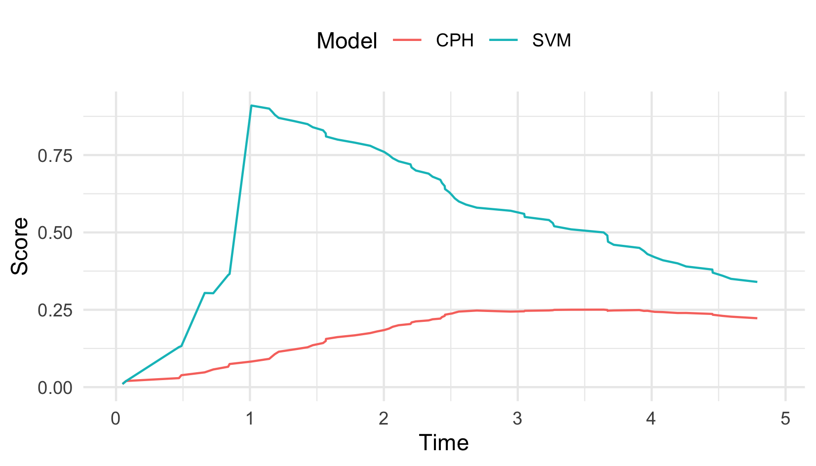
As well as evaluating probabilistic outcomes with integrated scoring rules, non-integrated scoring rules can be utilized for evaluating distributions at a single point. For example, instead of evaluating a probabilistic prediction with the ISBS over \(\mathbb{R}_{>0}\), one could compute the Brier score at a single time-point, \(\tau \in \mathbb{R}_{>0}\), only. Plotting these for varying values of \(\tau\) results in prediction error curves, which provide a simple visualization for how predictions vary over time. Prediction error curves are mostly used as a graphical guide when comparing few models, rather than as a formal tool for model comparison. Example prediction error curves are provided in Figure 8.2 for the ISBS where the Cox PH consistently outperforms the SVM.
8.4 Baselines and ERV
A common criticism of scoring rules is a lack of interpretability, for example, an ISBS of 0.5 or 0.0005 has no meaning by itself, so below we present two methods to help overcome this problem.
The first method is to make use of baselines for model comparison, which are models or values that can be utilized to provide a reference for a loss and provide a universal method to judge all models of the same class (Gressmann et al. 2018). In classification, it is possible to derive analytical baseline values, for example a Brier score is considered ‘bad’ if it is above 0.25 or a log loss if it is above 0.693 (Figure 8.1). This is because these are the values obtained if you always predicted probabilities as \(0.5\), which is the best un-informed (i.e., data independent) baseline in a binary classification problem. In survival analysis, simple analytical expressions are not possible as losses are dependent on the unknown distributions of both the survival and censoring time. For this reason it is advisable to include baseline models for model comparison. Common baselines include the Kaplan-Meier estimator (Section 3.5.2.1) and Cox PH (?sec-surv-models-crank). As a rule of thumb, if a model performs worse than the Kaplan-Meier, then it’s considered ‘bad’, whereas if it outperforms the Cox PH then it is considered ‘good’.
As well as directly comparing losses from a ‘sophisticated’ model to a baseline, one can also compute the percentage increase in performance between the sophisticated and baseline models, which produces a measure of explained residual variation (ERV) (Korn and Simon 1990; Korn and Simon 1991). For any survival loss \(L\), the ERV is,
\[ R_L(S, B) = 1 - \frac{L_{|S}}{L_{|B}} \]
where \(L_{|S}\) and \(L_{|B}\) are the losses computed with respect to predictions from the sophisticated and baseline models respectively.
The ERV interpretation makes reporting of scoring rules easier within and between experiments. For example, say in experiment A we have \(L_{|S} = 0.004\) and \(L_{|B} = 0.006\), and in experiment B we have \(L_{|S} = 4\) and \(L_{|B} = 6\). The sophisticated model may appear worse at first glance in experiment A (as the losses are very close) but when considering the ERV we see that the performance increase is identical (both \(R_L = 33\%\)), thus providing a clearer way to compare models.
8.5 Competing Risks
Similarly to discrimination measures, scoring rules are primarily used with competing risks by evaluating cause-specific probabilities individually (Geloven et al. 2022; Lee et al. 2018; Bender et al. 2021).
For example, given the cause-specific survival, \(S_e\), density, \(f_e\), and cumulative distribution function, \(F_e\), the right-censored log loss for event \(e\) is defined as
\[ L^e_{RCLL;i}(\hat{S}_{i;e}, t_i, \delta_i) = -\log[\delta_i\hat{f}_{i;e}(t_i) + (1-\delta_i)\hat{S}_{i;e}(t_i)] \]
Similar logic can be applied to the ISBS and other scoring rules.
Recently, an all-cause logarithmic scoring rule has been proposed which makes use of the IPC weighting in the ISBS (Alberge et al. 2025):
\[ L_{AC;i}(\hat{S}_i, t_i, \delta_i) = \sum^k_{e=1} \frac{\mathbb{I}(t_i \leq \tau, \delta_i = e)\log(\hat{F}_{i;e})}{\hat{G}(t_i)} + \frac{\mathbb{I}(t_i > \tau)\log(\hat{S}_i(\tau))}{\hat{G}(\tau)} \]
This ‘all-cause’ loss is an adaptation of the ISLL (Section 8.2.2) with the weights modified to handle competing risks. Comparing this loss to the decomposition in Section 8.2.1, the observations either: experience the event of interest, in which case their cause-specific CIF is evaluated; do not experience any event and so the all-cause survival is evaluated; or experience a different event and contribute nothing to the loss.
One advantage of the all-cause loss is that it provides a single scalar quantity, which makes it particularly convenient for (automated) model comparison, especially when there are many competing causes. However, this convenience comes at a cost as optimizing a single all-cause loss can obscure heterogeneity in performance across causes. This is especially problematic when accurate modeling of some causes is more important than others. Moreover, a model may achieve good overall performance while substantially underperforming for a clinically important cause. As a result, when performance for individual causes is a priority, cause-specific scoring rules may be preferable. In such settings, automated procedures, such as those used for hyperparameter optimization (Chapter 2), would require multi-objective optimization methods (Morales-Hernández et al. 2023).