4 Event-history Analysis
This page is a work in progress and major changes will be made over time.
In this chapter we take a more general view on time-to-event data. So far, we only considered a single potentially censored, outcome of interest. Here we explore more complex settings with multiple, potentially mutually exclusive events and recurrences of events. In this generalization, the observed data is sometimes referred to as event-history data and its analysis as event-history analysis.
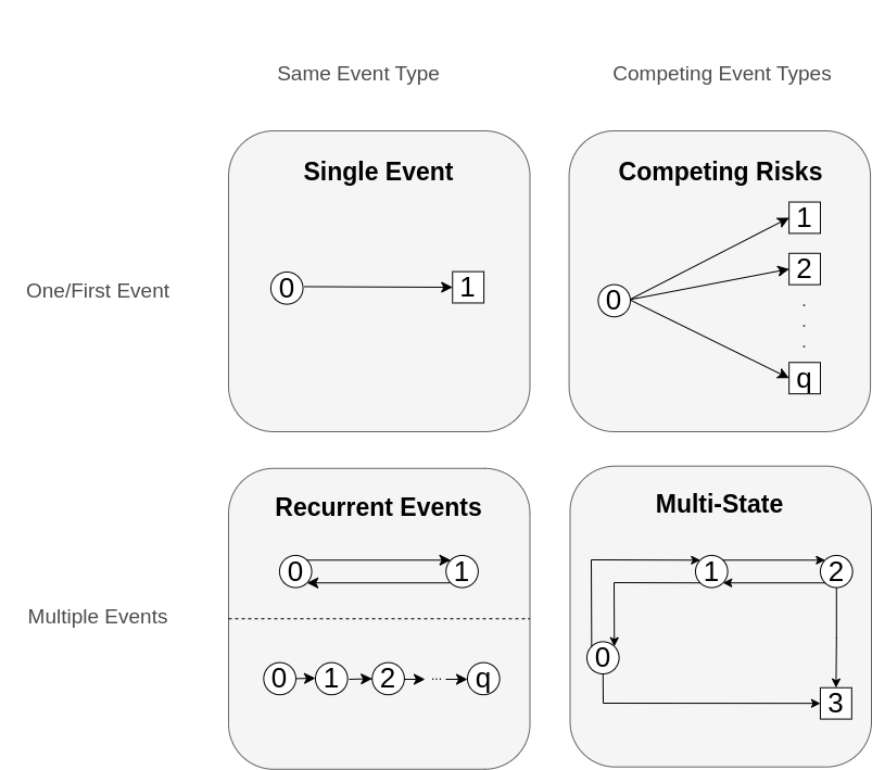
One way to think about event history data is in terms of transitions between different states, as illustrated in Figure 4.1. Usually, a subject starts out in an initial state \(0\) (for example, ‘healthy’) and from there transitions to different states. States from which further transitions are possible are called transient (displayed as circles), otherwise a state is called terminal or absorbing (displayed as squares).
In the single event setting (Figure 4.1, upper left panel), a subject can only transition to one state (the event of interest). This setting was the focus of Chapter 3. There, the censoring event was considered independent of the event of interest. In the competing risks setting (Figure 4.1, upper right panel, Section 4.2), a subject could transition to any of the \(q\) mutually exclusive states, thus the subject is initially at risk for a transition to multiple states. Once one of them occurs, the process is considered to have concluded (for the modeling purposes).
In the recurrent events setting (Figure 4.1 lower left panel), the same event can be observed multiple times on the same subject (for example recurrent respiratory infections during one year). Two different ways to represent recurrent events are shown: (top) reset the status to \(0\) after occurrence of an event or (bottom) consider the \(1\)st, \(2\)nd, etc. recurrences of the event as separate states. A detail omitted in the graph: Often recurrent event processes also have a competing, absorbing event. In this more complex setting, but also in general, recurrent events are often represented as multi-state process, which we discuss next. Therefore we forgo detailed discussion of this setting in this book and refer to Cook and Lawless (2007) for a detailed account specific to recurrent events analysis.
In the most general case, the multi-state setting (Figure 4.1 lower right panel, Section 4.3), there are multiple transient and terminal states with potential back transitions (for example, moving between different stages of an illness with the possibility of (partial) recovery and death as terminal event).
Note that the concepts discussed in Section 3.3 and Section 3.4 are still relevant here, as, dependent on the specific process, any transition between two states could be subject to different types of censoring and truncation. In particular, remaining in one of the transient states until the end of follow-up constitutes right-censoring with respect to all possible transitions from that state and left-truncation is particularly important as subjects enter the risk sets for a transition at different time points in context of recurrent events and multi-state settings.
4.1 A process point of view
In order to formalize the different settings more conveniently, we introduce the stochastic process \[ E(\tau) \in \{0,\ldots, q\},\ \tau \geq 0, \tag{4.1}\] which indicates the state that is occupied at time \(\tau\).
Using this notation in the single-event setting we get \(E(\tau) \in \{0,1\}\) such that the hazard 3.2 could be written as \[ \begin{aligned} h(\tau) &= \lim_{\mathrm{d}\tau\searrow 0}\frac{P(Y \in [\tau, \tau + \mathrm{d}\tau)|Y \geq \tau)}{\mathrm{d}\tau}\\ & = \lim_{\mathrm{d}\tau\searrow 0}\frac{P\left(E(\tau + \mathrm{d}\tau)=1|E(\tau-)=0\right)}{\mathrm{d}\tau}, \end{aligned} \tag{4.2}\] where \(\tau-\) indicates the time point immediately before \(\tau\).
This notation doesn’t yield many advantages in the single-event setting, but will shorten notation later on, particularly in the multi-state setting. While not further pursued here beyond notational convenience, we refer to Aalen et al. (2008) for an excellent treatment of event-history analysis derived from the point of view of stochastic processes.
4.2 Competing Risks
In contrast to single-event survival analysis, competing risks are concerned with the time to the first of multiple, mutually exclusive events.
Table 4.1. shows an excerpt of the sir.adm data (Allignol et al. 2008) of patients on an intensive care unit (ICU). Time under observation (time) could end in one of three outcomes: \(1\) (discharge alive), \(2\) (death on ICU) or \(0\) (neither discharge nor death at the end of follow-up, which constitutes right-censoring at the end of study). The interest was in how pneumonia status (pneumonia) at admission to the ICU affects mortality.
sir.adm dataset (Allignol et al. 2008). Each row represent one subject,time is the time under observation, status indicates the outcome observed (\(0\): censored at the end of the study, \(1\): discharged alive from the ICU, \(2\): death in the ICU). pneumonia indicates whether a subject already had pneumonia at ICU admission.
time |
status |
pneumonia |
|---|---|---|
| 8 | 0 | no |
| 8 | 0 | no |
| 31 | 1 | yes |
| 5 | 1 | no |
| 9 | 2 | no |
| 5 | 2 | no |
Contrast this data to the tumor data example in Section 3.5.2.1. There, patients were followed even after hospital discharge, thus loss to follow-up could be considered reasonably independent of the event of interest (death). In this study, follow-up stopped once patients were discharged. As discharged patients are healthier compared to the ones who remain on ICU, assuming independence between the time until discharge and time until death is unrealistic. Analysis of this data and how the different assumptions (independent censoring vs. competing risks) affects the estimates is discussed in Section 4.2.2 and Section 4.2.4.
4.2.1 Notation and Definitions
In the competing risks setting, everyone starts out in the initial state \(0\) and can progress to one of the absorbing states
\[ e \in \{1,\ldots,q\} \tag{4.3}\]
These absorbing states are also often refered to as competing events, event types, or causes (as in cause that ended the observation). State \(e = 0\) is the initial state and a subject that remains in state \(0\) until the end of the follow up is considered censored.
The goal is to characterize the process \(E(\tau) \in \{0,\ldots, q\}\) in terms of transition hazards and probabilities. In extension of 4.2, we define cause-specific hazards \[ h_{e}(\tau) = \lim_{\mathrm{d}\tau\to 0} \frac{P(E(\tau + \mathrm{d}\tau) = e\ |E(\tau-)=0)}{\mathrm{d}\tau}. \tag{4.4}\] Analogous to the single-event case, we can also define the cause-specific cumulative hazard \[ H_{e}(\tau) = \int_{0}^\tau h_e(u)\ du \tag{4.5}\] As competing events are mutually exclusive at any time \(\tau\), it is possible to define the all-cause hazard which is the hazard of any event occurring as the sum of all cause-specific hazards \[ h(\tau) = \sum_{e = 1}^{q}h_{e}(\tau), \tag{4.6}\] as well as the all-cause cumulative hazard, which can be obtained either via the integral over the all-cause hazard (4.6) or as sum of cause-specific cumulative hazards (4.5):
\[ \begin{aligned} H(\tau) & = \sum_{e=1}^q H_{e}(\tau) = \sum_{e=1}^{q}\int_{0}^\tau h_{e}(u)\ du\\ & =\int_{0}^\tau \sum_{e=1}^{q} h_{e}(u)\ du = \int_{0}^\tau h(u)\ du \end{aligned} \tag{4.7}\]
The all-cause survival probability gives the probability that none of the events occurred before \(\tau\). This is usually not estimated directly but calculated from the cause specific hazards instead via 4.7 and 4.8:
\[ S(\tau) = P(Y > \tau) = \exp(-H(\tau)) \tag{4.8}\]
Finally, the probability of experiencing an event \(e\) before time \(\tau\), which is often referred to as Cumulative Incidence Function (CIF), is given by \[ \begin{aligned} F_{e}(\tau) &= P(Y \leq \tau, E(Y) = e) &\ \\ & = \int_{0}^\tau f_e(u)\ \mathrm{d}u = \int_{0}^\tau S(u-)h_{e}(u)\ \mathrm{d}u, \end{aligned} \tag{4.9}\] where
- \(S(u-)\) is the probability of surviving (not experiencing any of the competing events) until the time-point shortly before \(u\)
- \(f_e(u)\mathrm{d}u = S(u-)h_{e}(u)\mathrm{d}u\) is the probability of experiencing event \(e\) at time point \(u\) (which follows analogously to 3.2).
Note that here we use the notation \(S(u-)\) rather than \(S(u)\) to make explicit that we want the probability to survive until the time point immediately before \(u\). This doesn’t make much difference in continuous time where \(P(T > t) = P(T\geq t)\), but may be important in (discrete) approximations (as in Section 4.2.2).
\(F_e(\tau)\) can be interpreted as the proportion of subjects who experienced event of type \(e\) until time \(\tau\). Because the events are mutually exclusive, it holds that \[ S(\tau) + \sum_{e=1}^q F_e(\tau) = S(\tau) + F(\tau)= 1 \] where \(F(\tau)\) is the probability that an event of any type occurring before \(\tau\) and \(S(\tau)\) the probability that no event occurs (4.8).
Note that all terms of 4.9 can be calculated from the individual hazards (4.4). Many estimation procedures for the CIF take this approach, consequently referred to as cause-specific hazards approach.
4.2.2 Non-parametric estimators
Non-parametric estimators for the cause-specific (cumulative) hazard (4.5) in the competing risks setting are derived analogously to the single event case (Section 3.5.2). The non-parametric estimate for the CIF is obtained by plugging in the non-parametric estimates of \(S(t)\) and \(h(t)\) into (4.9) as follows.
First, recall from Section 3.2 the definitions of the unique ordered event times \(t_{(k)}, k=1\ldots,m\), the risk-set at time \(t_{(k)}\), \(\mathcal{R}_{t_{(k)}}\), the number of events, \(d_{t_{(k)}}\), and number of observations at risk \(n_{t_{(k)}}\). Assume partitioning of the follow-up into \(m\) disjoint intervals \((t_{(k-1)}, t_{(k)}],k=1,\ldots,m\), such that \(Y\in (t_{(k-1)}, t_{(k)}] \Leftrightarrow \tilde{Y}=t_{(k)}\), with \(\tilde{Y}\) defined as in Section 3.1.2.
An estimate for the cause-specific hazard is derived by updating the numerator in 3.14 to \(d_{e,t_{(k)}}\) (the number of events of type \(e\) at time \(t_{(k)}\)): \[ h^d_{e}(t_{(k)}) := \frac{d_{e,t_{(k)}}}{n_{t_{(k)}}},\ e \in \{1, \ldots, q\}. \tag{4.10}\]
Finally, the Aalen-Johansen (AJ) estimator (Aalen and Johansen (1978)) for the CIF is obtained by plugging in the Kaplan-Meier estimate (3.15) for the all-cause survival probability (probability that none of the competing events occurred) and the cause-specific hazard (4.10) for cause \(e\) into (4.9): \[ F_{AJ,e}(\tau) = \sum_{k:t_{(k)}\leq \tau} \hat{S}_{KM}(\tau-)\hat{h}^d_e(\tau)= \sum_{k:t_{(k)}\leq \tau} \hat{S}_{KM}(t_{(k-1)})\frac{d_{e,t_{(k)}}}{n_{t_{(k)}}} \tag{4.11}\]
4.2.3 Application to mortality of ICU patients
For illustration of the AJ estimator and the interpretation of the CIFs consider the analysis conducted in Beyersmann et al. (2012), based on the data from Table 4.1. Recall that one is interested in estimation of the mortality conditional on pneumonia status at admission, while accounting for discharge from the ICU as competing risk (\(E(\tau) \in \{0,1,2\}\), where \(0\) indicates being alive in ICU (the initial state), \(1\) indicates discharge from ICU and \(2\) indicates death). While the AJ estimator cannot naturally incorporate feature information, it can be applied to subgroups of the data (here based on the pneumonia status \(x_{\text{pneu}} \in \{0,1\}\)). Note that this will yield different sets of unique event times in each group, thus the AJ can have jumps at different time-points for the two groups.
Figure 4.2 shows the AJ estimates of the CIFs for each event type (discharge/death) stratified by pneumonia status. For example, the proportion of subjects with pneumonia being discharged until \(\tau=120\text{ days}\) is approximately 75% (\(\hat{F}_{1}(120|x_{\text{pneu}}=1) = \hat{P}(Y \leq 120, E(Y) = 1|x_{\text{pneu}}=1)\approx 0.75\)), while approximately 25% died in the ICU (\(\hat{F}_{2}(120|x_{\text{pneu}}=1) = \hat{P}(Y \leq 120, E(Y) = 2|x_{\text{pneu}}=1)\approx 0.25)\). For patients without pneumonia we have \(\hat{F}_{1}(120|x_{\text{pneu}}=0) \approx 0.91\) and \(\hat{F}_{2}(120|x_{\text{pneu}}=0) \approx 0.09\). In this example, \(\hat{F}_{1} + \hat{F}_{2} \approx 1\) for both pneumonia groups, as only 14 of 747 patients were censored (neither discharge nor death) at the end of the follow-up and thus the all-cause survival probability \(\hat{S}(120) \approx 0\).
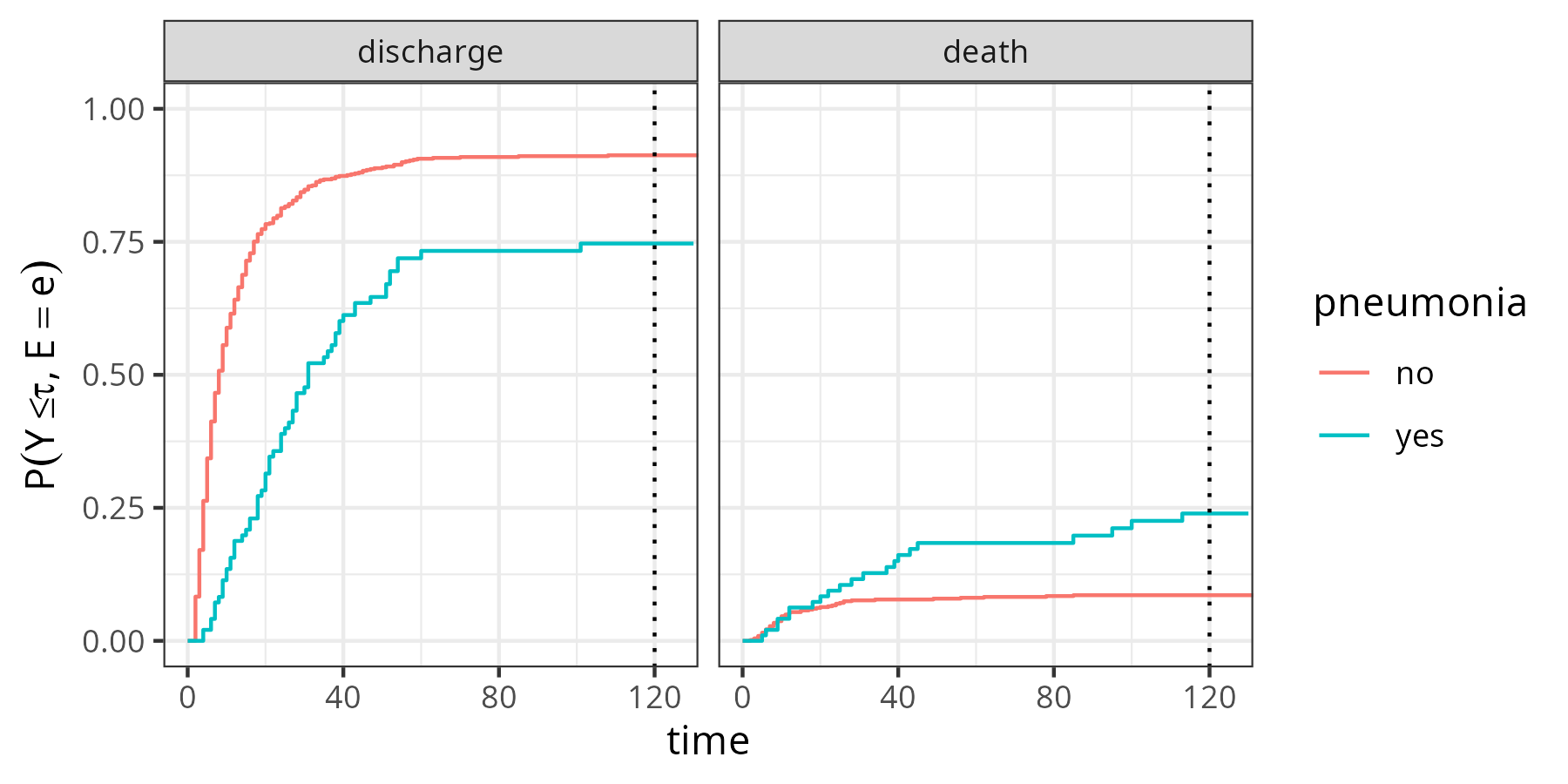
sir.adm data (Allignol et al. 2008), stratified by pneumonia status at admission to the ICU. Left panel: Proportion of subjects discharged alive from the ICU. Right panel: Proportion of subjects who died in the ICU.
4.2.4 Independent Censoring vs. Competing Risks
It is worth spending some time to consider the difference between independent right-censoring and competing risks. Note that for the estimation of the hazard (4.10), occurrences of competing events are implicitly assumed right-censored (as \(d_{e,t_{(k)}}\)) only counts events of type \(e\) and \(n_{t_{(k)}}\) contains the same subjects that would remain if events of type \(\tilde{e}\neq e\) were considered censored before \(t_{(k)}\). Nevertheless, competing risks are taken into account in the definition of the CIFs (4.9) and thus also in the AJ estimator (4.11), as the all-cause survival probability (4.8) depends on all cause-specific hazards.
In contrast, assume that in our analysis of the sir.adm data we would consider time of discharge as independent right-censoring. As we only have one other event (death), the data could be treated as single-event, right-censored data as in Chapter 3 and therefore analyzed using the Nelson-Aalen estimator (3.17). The probability of death before some time-point \(\tau\) could thus be obtained via \(P(Y\leq \tau) = F(\tau) = 1 - S_{NA}(\tau)\).
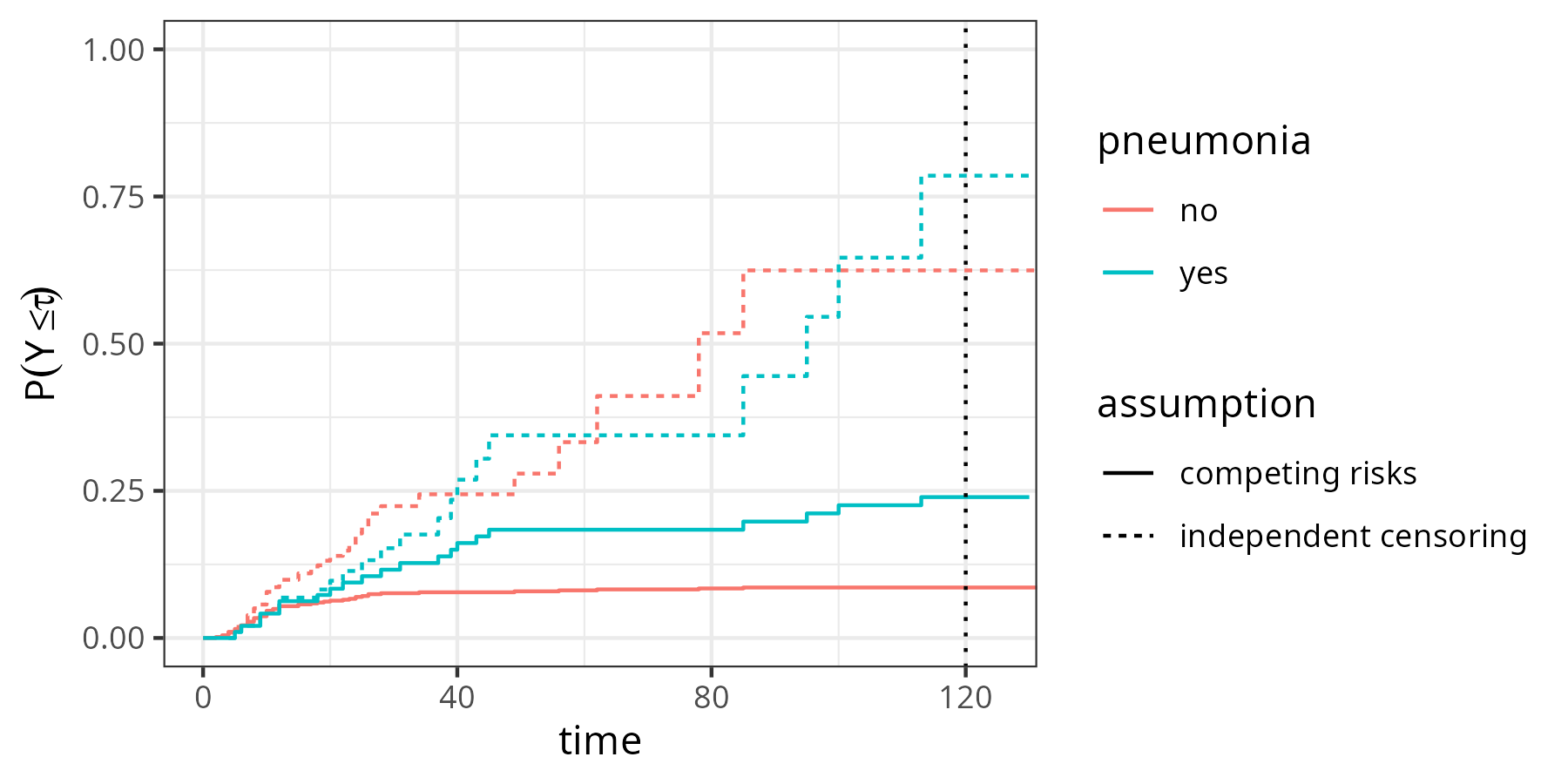
Figure 4.3 shows the estimates obtained under the two assumptions. Solid lines indicate the probabilities under the competing risks assumption (identical to the right-hand side of Figure 4.2). Dashed lines are obtained under the independent right-censoring assumption. Clearly, the probabilities of dying at time \(\tau=120\) are greater when independent censoring is assumed (\(\approx\) 75% vs. \(\approx\) 25% in the pneumonia group and \(\approx\) 62% vs. \(\approx\) 13% in the no pneumonia group).
4.3 Multi-state Models
The multi-state process can be considered the most general type of time-to-event process, as other types (single-event, competing risks, recurrent events) can be viewed as special cases. Multi-state modeling allows realistic depiction of complex processes where subjects can start in different states and transition back and forth between them.
For illustration consider the prothr dataset (de Wreede et al. 2011) of liver cirrhosis patients from a randomized clinical trial with possible transitions depicted in Figure 4.4. Patients may have normal (state \(0\)) or abnormal (state \(1\)) levels of prothrombin (a protein important for blood clotting, produced by the liver) at the beginning of the trial. Some patients where treated with prednisone (which suppresses immune response and reduces inflammation) and others received a placebo. Death (state \(2\)) constitutes an absorbing state.
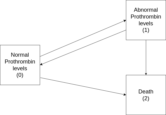
The goal of the trial was to investigate if treatment (prednisone) slows down or reverses disease progression (transitions \(0 \rightarrow 1\) and \(1 \rightarrow 0\)) and reduces mortality (transitions \(0 \rightarrow 2\) and \(1 \rightarrow 2\)).
Table 4.2 shows a subset of the data set and contains for each subject (id)one row for each transition for which the subject was at risk for. In this example, this includes transitions that were possible, but didn’t happen (counterfactual transitions). The columns from and to indicate the initial state and the possible end state. tstart indicates the time at which the subject entered the risk set for said transitions and tstop the time point at which the subjects exited the from state (or were censored for any transition). The variable status indicates whether the transition was actually made (status = 1) or not (status = 0). This is necessary, as all possible transitions are listed, so we need an indicator for which transition actually occurred. If status=0 for all possible transitions, the subject is censored for further transitions. Finally, treatment indicates whether a patient was assigned the treatment or placebo group.
Concretely, subject id=1 already had abnormal prothrombin levels at the beginning of the trial, thus started in state \(1\) with possible transitions \(1\rightarrow 0\) and \(1 \rightarrow 2\). In this case, the patient died, thus transition \(1\rightarrow 2\) was realized after 151 days, while the transition \(1 \rightarrow 0\) is a ‘counterfactual’ transition that could have happened in the time-span between tstart=0 and tend=151, but didn’t. Patient id=8 also started in state \(1\), but made a back transition to normal prothrombin levels after 211 days at which time they entered the risk set for transitions \(0\rightarrow 1\) and \(0\rightarrow 2\). Neither of the transitions occurred, as status=0 for both transitions, which means the subject remained in status \(0\) until the end of their follow-up at 2770 days (that is was right-censored at 2770 days). Finally, subject id=46 started in state 0 (normal prothrombin levels), transitioned to state 1 (abnormal levels) after 415 days and then died (transition \(1\rightarrow 2\)) two days later. This also illustrates the importance of left-truncation (Section 3.4) in multi-state processes. For example, subjects id=1 and id=8 are at risk for the transitions \(1 \rightarrow 0\) and \(1 \rightarrow 2\) from the beginning of the trial (tstart = 0). Subject id=46 on the other hand starts in state 0 and only enters state \(1\) (and thus the risk set for the transitions \(1\rightarrow 0\) and \(1\rightarrow 2\)) after 415 days (tstart = 415). Other subjects in the data may never enter the risk set for these transitions by remaining in state 0 until the end of follow up or by directly transitioning to state \(2\). The fact that subjects enter the risk sets for different transitions at different time points technically constitutes left-truncation and thus should be taken into account accordingly (Section 4.3.4).
prothr dataset (de Wreede et al. 2011).
| id | from | to | trans | tstart | tstop | status | treatment |
|---|---|---|---|---|---|---|---|
| 1 | 1 | 0 | 3 | 0 | 151 | 0 | Placebo |
| 1 | 1 | 2 | 4 | 0 | 151 | 1 | Placebo |
| 8 | 1 | 0 | 3 | 0 | 211 | 1 | Prednisone |
| 8 | 1 | 2 | 4 | 0 | 211 | 0 | Prednisone |
| 8 | 0 | 1 | 1 | 211 | 2770 | 0 | Prednisone |
| 8 | 0 | 2 | 2 | 211 | 2770 | 0 | Prednisone |
| 46 | 0 | 1 | 1 | 0 | 415 | 1 | Prednisone |
| 46 | 0 | 2 | 2 | 0 | 415 | 0 | Prednisone |
| 46 | 1 | 0 | 3 | 415 | 417 | 0 | Prednisone |
| 46 | 1 | 2 | 4 | 415 | 417 | 1 | Prednisone |
4.3.1 Notation and Definitions
In the competing risks setting, we characterized the data generating process by cause-specific transitions hazards \(h_e(\tau)\) (4.4). Implicitly these are transitions from starting state \(0\) to end state \(e\), however, since everyone starts in state \(0\) this is ignored notationally. In the multi-state setting on the other hand, subjects can be in different states at different time points. Transitions between different states are therefore characterized by transition-specific hazards, denoted by \(h_{\ell\rightarrow e}(\tau)\) or short \(h_{\ell e}(\tau)\), where \(\ell\) is the starting state and \(e\) the end state.
Let \(E(\tau)\in \{0,\ldots,q\}\) be the state of the process at time \(\tau\) as before (4.1). Then, the transition-specific hazard can be defined as \[ h_{\ell e}(\tau) = \lim_{\mathrm{d}\tau\to 0} \frac{P(E(\tau + \mathrm{d}\tau)=e|E(\tau-) = \ell)}{\mathrm{d}\tau} \tag{4.12}\]
Transition hazards 4.12 indicate the instantaneous risk to enter state \(e\) at time \(\tau\) given occupation of state \(\ell\) at \(\tau-\), which is the instant before \(\tau\).
Analogous to the competing risks setting, we can define the transition specific cumulative hazards
\[ H_{\ell e}(\tau) = \int_{0}^{\tau}h_{\ell e}(u)du \tag{4.13}\]
The probability to transition from state \(\ell\) to \(e\) between two time-points depends on all transitions possible from \(\ell\) and potentially the transitions that have taken place in the past. Thus, other quantities of interest in the multi-state setting are the transition probabilities \(P_{\ell e}(\zeta, \tau):= P(E(\tau) = e|E(\zeta) = \ell)\), that is the probability to transition from state \(\ell\) to state \(e\) between time points \(\zeta < \tau\). Implicitly, this notation assumes that the process is Markovian: the transition probability depends only on the state at \(\zeta\) and not any additional past states. Extensions do exist that relax this assumption, for example by including information about the past, but are not relevant for now.
Transition probabilities of a multi-state process are often summarized in a matrix \[ \mathbf{P}(\zeta, \tau):= \begin{pmatrix} P_{00}(\zeta, \tau) & \cdots & P_{0q}(\zeta, \tau)\\ \vdots & \ddots & \vdots\\ P_{q0}(\zeta, \tau) & \cdots & P_{qq}(\zeta, \tau)\\ \end{pmatrix}, \tag{4.14}\] where rows indicate starting states and columns indicate end states. Some of the elements of \(\mathbf{P}\) might be zero or one depending on the specific process, presence of absorbing states and possible pathways between states. As subjects can only be in one of the \(q+1\) states at \(\tau\), rows sum to \(1\): \[ \sum_{e =0}^q P_{\ell e} = 1,\forall \ell \in \{0, \ldots,q\}. \tag{4.15}\]
4.3.2 Transition probabilities
In this section we briefly motivate how transition probabilities between two non-consecutive time points can be expressed as the product (integral) of transition probabilities between intermediate, subsequent time points.
For illustration, consider what is often referred to as an illness-death model depicted in Figure 4.5 (similar to Figure 4.4, but without back-transition), where subjects can transition from healthy state \(0\) to absorbing death state \(2\) either directly or via intermediate state \(1\).
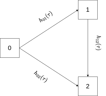
In this example, back-transitions are not possible, therefore the lower triangle of the matrix is filled with zeros and \(P_{22}(\zeta, \tau) = 1, \forall\ \zeta < \tau\) by virtue of being an absorbing state. The matrix of transition probabilities is thus given as \[ \mathbf{P}(\zeta, \tau) = \begin{pmatrix} P_{00}(\zeta, \tau) & P_{01}(\zeta, \tau) & P_{02}(\zeta, \tau)\\ 0 & P_{11}(\zeta, \tau) & P_{12}(\zeta, \tau)\\ 0 & 0 & 1\\ \end{pmatrix} \tag{4.16}\] First, assume that data is collected in discrete time, that is \(\zeta, \tau \in \{0, 1, 2,\ldots\}, \zeta < \tau\) and transitions only occur at these discrete time points and not in between. Say we are interested in transition probability \(P_{02}(4, 6)\), that is the probability to transition from state \(0\) to state \(2\) between time points \(\zeta=4\) and \(\tau=6\), given we are in state \(0\) at time \(\zeta = 4\). This is possible in the three ways depicted in Figure 4.6.
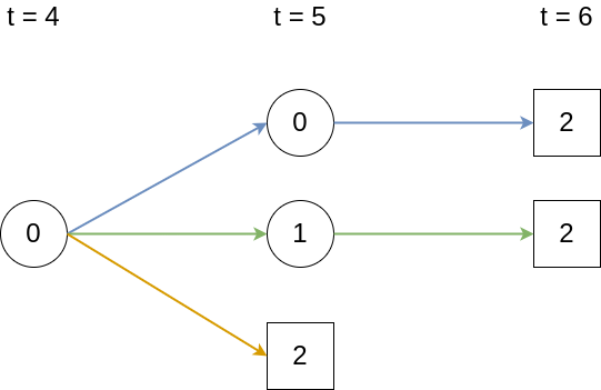
Thus, \(P_{02}(4,6) = \textcolor{blue}{p_{00}(5)p_{02}(6)} + \textcolor{green}{p_{01}(5)p_{12}(6)} + \textcolor{orange}{p_{02}(5)}\), where \(p_{\ell e}(\tau)=P(E(\tau)=e|E(\tau -1) = \ell)\) are the probabilities for transitions \(\ell \rightarrow e\) between two subsequent discrete time points. Thus, in discrete time, the matrix of transition probabilities can be represented as a finite matrix product
\[ \mathbf{P}(\zeta, \tau) = \prod_{j =\zeta+1}^{\tau} \begin{pmatrix} p_{00}(j) & p_{01}(j) & p_{02}(j)\\ 0 & p_{11}(j) & p_{12}(j)\\ 0 & 0 & 1\\ \end{pmatrix}. \tag{4.17}\]
For the concrete example we thus have
\[ \begin{aligned} \mathbf{P}(4, 6) &= \begin{pmatrix} P_{00}(4, 6) & P_{01}(4, 6) & P_{02}(4, 6)\\ 0 & P_{11}(4, 6) & P_{12}(4,6)\\ 0 & 0 & 1 \end{pmatrix} = \prod_{j=5}^6 \begin{pmatrix} p_{00}(j) & p_{01}(j) & p_{02}(j)\\ 0 & p_{11}(j) & p_{12}(j)\\ 0 & 0 & 1 \end{pmatrix}\\ & = \begin{pmatrix} p_{00}(5) & p_{01}(5) & p_{02}(5)\\ 0 & p_{11}(5) & p_{12}(5)\\ 0 & 0 & 1 \end{pmatrix} \begin{pmatrix} p_{00}(6) & p_{01}(6) & p_{02}(6)\\ 0 & p_{11}(6) & p_{12}(6)\\ 0 & 0 & 1 \end{pmatrix}\\ &= \begin{pmatrix} p_{00}(5) p_{00}(6) & p_{00}(5)p_{01}(6) + p_{01}(5)p_{11}(6) & p_{00}(5)p_{02}(6) + p_{01}(5)p_{12}(6) + p_{02}(5)\\ 0 & p_{11}(5) p_{11}(6)& p_{11}(5)p_{12}(6) + p_{12}(5)\\ 0 & 0 & 1 \end{pmatrix}, \end{aligned} \]
where the quantity of interest, \(P_{02}(4, 6)\) is given in the top right corner, but other transition probabilities are also readily available. For example, the probability to transition from state \(1\) to \(2\) between time points \(\zeta=4\) and \(\tau=6\) is given as \(P_{12}(4, 6) = p_{11}(5)p_{12}(6) + p_{12}(5)\).
Returning to the continuous time setting where transitions can occur at any time point, ideas from the discrete time setting still hold. Imagine dividing the interval \((\zeta, \tau]\) into \(J\) intervals such that \(\zeta = t_{0} < t_{1} < \cdots < t_{j} < \cdots t_{J} = \tau\), assuming that no events occur between time points \(t_{j} \in \mathbb{R}_+, j=1,\ldots, J\). Then 4.17 still holds when replacing \(p_{\ell e}(j)\) with \(p_{\ell e}(t_j)\).
4.3.3 Transition probabilities and hazards
Increasing the number of intervals to infinity or equivalently, reducing the interval size to infinitesimally small intervals we can define the transition probability matrix as a product integral over the instantaneous transition probabilities \(p_{\ell e}(u)\), expressed in terms of transition-specific (cumulative) hazards.
To do so, we use, somewhat informally, the following relationships
- From equations 4.12 and 4.13 we can equate the instantaneous transition probabilities to increments of the cumulative hazard (that is the increase in the cumulative hazard within a (fixed, infinitesimally) small interval \(\mathrm{d}u\)): \(dH_{\ell e}(u) = P\big(E(u+du)=e|E(u-) = \ell\big) =: p_{\ell e}(u)\),
- because of relationship 4.15, diagonal elements (transitions into the same state) are set to \(dH_{\ell \ell}(u) := -\sum_{e \neq \ell} dH_{\ell e}(u)\) such that \(1 + dH_{\ell\ell}(u) = 1-\sum_{e \neq \ell} dH_{\ell e}(u) = 1 - \sum_{e\neq \ell}p_{\ell e}(u) = p_{\ell\ell}(u)\).
Consequently, the transition probability matrix can be written as \[ \begin{aligned} \mathbf{P}(\zeta, \tau) &= \mathscr{P}_{u \in (\zeta, \tau]} \begin{pmatrix} p_{00}(u) = 1 + dH_{00}(u) & \cdots & p_{0q}(u) = dH_{0q}(u)\\ \vdots & \ddots & \vdots\\ p_{q0}(u) = dH_{q0}(u) & \cdots & p_{qq}(u) = 1 + dH_{qq}(u)\\ \end{pmatrix}\nonumber\\ & \ \\ & = \mathscr{P}_{u \in (\zeta, \tau]}(\mathbf{I} + d\mathbf{H}(u)),\nonumber\\ \end{aligned} \tag{4.18}\] where \(\mathscr{P}\) is the product integral operator, \(\mathbf{I}\) is a \((q+1) \times (q+1)\) identity matrix and \(d\mathbf{H}(u)\) is the matrix of increments of the cumulative hazard within infinitesimally small intervals. Thus, similar to the competing risks setting, relationship 4.18 implies that knowledge of the transition specific (cumulative) hazards is sufficient to fully specify the multi-state process.
As analytical solutions of 4.18 only exist for specific models, in practice, the transition probabilities are often once again approximated numerically via a finite matrix product on a discrete time grid \(\zeta = t_0 < t_1 < \cdots < t_{J-1} < t_{J} = \tau\) \[ \mathbf{P}(\zeta, \tau) \approx \prod_{j=1}^{J}(\mathbf{I} + \triangle\mathbf{H}_{\ell e}(t_{j})), \tag{4.19}\] where \(\triangle H_{\ell e}(t_{j}) = H_{\ell e}(t_{j}) - H_{\ell e}(t_{j-1})\) is the increment of the cumulative hazards between to consecutive time points.
4.3.4 Non-parametric estimation of transition probabilities
From 4.19, it follows that transition probabilities can be estimated by first computing the transition-specific cumulative hazards, \(H_{\ell e}(\tau)\). Similarly to the competing risks setting (Section 4.2.2), we can first define the transition specific hazards \[ h^{d}_{\ell e}(t_{(k)}):= \frac{d_{\ell e,t_{(k)}}}{n_{\ell; t_{(k)}}}, \] where
- \(d_{\ell e,t_{(k)}}\) is the number of subjects that made the transition \(\ell \rightarrow e\) at time \(t_{(k)}\) and
- \(n_{\ell; t_{(k)}}\) is the number of subjects in state \(\ell\) immediately before \(t_{(k)}\).
The cumulative transition-specific hazards follow as \[ H_{NA,\ell e}(\tau) = \sum_{k:t_{(k)}\leq \tau} h^d_{\ell e}(t_{(k)}) = \sum_{k:t_{(k)}\leq \tau}\frac{d_{\ell e,t_{(k)}}}{n_{\ell; t_{(k)}}}, \]
and transition probabilities are obtained via 4.19 as \[ \mathbf{P}(\zeta, \tau) = \prod_{j=1}^{J}\big(\mathbf{I} + \triangle\mathbf{H}_{NA,\ell e}(t_{(j)})\big). \tag{4.20}\]
4.3.5 Application to liver cirrhosis patients
For illustration, consider again the prothr data set (Table 4.2), with possible transitions summarized in Figure 4.4. In contrast to the illness-death model in Figure 4.5, back transitions are possible and some subjects already start in the “abnormal” state at the beginning of the study.
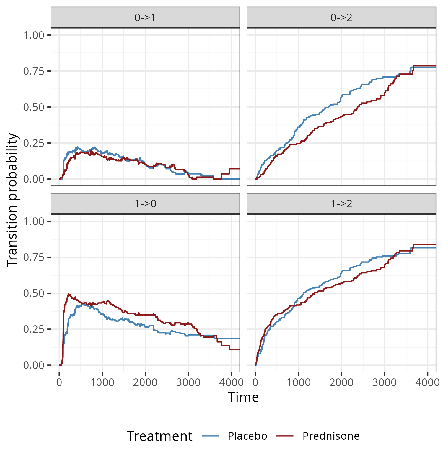
Figure 4.7 shows the transition probabilities for the four possible transitions over time for subjects who received treatment and placebo, respectively. In this example back-transitions are possible, therefore, in contrast to the cumulative incidence functions in the competing risks setting, transition probabilities (to transient states) are not monotonously increasing over time. While the probabilities to transition from normal or abnormal state to death (\(0 \rightarrow 2\), \(1 \rightarrow 2\)) increase over time for both groups, probabilities for transitions between the transient states (normal to abnormal and vice versa) increase in the beginning but eventually decreases over time. Overall, prednisone doesn’t appear to have a strong protective effect. Although there appears to be a reduction in \(0 \rightarrow 2\) transitions and an increase in \(1\rightarrow 0\) transitions between time points \(1000\) and \(3000\), this effect doesn’t seem to persist until the end of the follow up.