17 Pseudo-value regression
This page is a work in progress and minor changes will be made over time.
Pseudo-value based approaches have been introduced in the survival analysis community quite recently (see Andersen and Pohar Perme (2010) for an overview), but have gained popularity ever since due to their flexibility and ease of application. Similar to the IPCW based reduction (Chapter 16). After data transformation, they allow the application of arbitrary regression learners for uncensored data in order to estimate a quantity of interest (like the survival probability, restricted mean survival time, cumulative incidence function, etc.) conditional on features. It’s a two step approach where
- a jackknife (leave-one-out) procedure based on univariate (featureless) estimators for the quantity of interest is used to calculate pseudo-values, which are defined for all subjects in the data, regardless of their censoring status.
- the calculated pseudo-values are used as outcome in a regression task (Section 2.2.1) to learn a function that maps the features to the pseudo-values. Predictions from the model are conditional predictions of the quantity of interest.
Formally, let \(\psi(\tau|\mathbf{x})\) denote some quantity of interest, for example the survival probability \(S(\tau | \mathbf{x})\) or the restricted mean survival time, \(\text{RMST}(\tau | \mathbf{x})\). Let \(\psi(\tau)\) be an univariate (featureless), unbiased estimator of the quantity of interest based on all observations and \(\psi^{-i}(\tau)\) be an unbiased estimator of the same quantity obtained by omitting the \(i\)-th observation from the data set (for example \(S_{KM}(\tau)\) and \(S_{KM}^{-i}(\tau)\) for the survival probability). Let \(n\) the size of the data set. Pseudo-values are defined by \[ \theta_i(\tau) = n\psi(\tau) - (n-1)\psi^{-i}(\tau). \tag{17.1}\]
Thus, the calculation of the pseudo-values requires \(n+1\) estimates of the univariate estimator \(\psi(\tau)\) per time point \(\tau\) (\(n\) estimates omitting each observation in the data set plus one for the overall estimate). This may seem prohibitive, but calculation of univariate estimators is usually fast and methods that use efficient approximations have been proposed in the literature (Parner et al. (2023), Bouaziz (2023)). Also, pseudo-value analysis is usually used when the interest lies in estimation at one or few time points \(\tau\) rather than the entire event time distribution.
An important property of pseudo-values is that their expectation conditional on features \(\mathbf{x}_i\) is equal to the quantity of interest, that is \[ E(\theta_i(\tau|\mathbf{x}_i)) = \psi(\tau|\mathbf{x}_i). \tag{17.2}\] In order to learn the relationship of features with the quantities in (17.2), the pseudo-values are regressed on the features \(\mathbf{x}_i\) by specifying \[ E(\theta_i(\tau|\mathbf{x}_i)) = h(f_{\tau}(\mathbf{x}_i)), \tag{17.3}\] where \(f_{\tau}(\mathbf{x}_i)\) is a function of the features \(\mathbf{x}_i\) (for example \(f_{\tau}(\mathbf{x}) = \mathbf{x}^\top\boldsymbol{\beta}_{\tau}\)) that is learned by the model and \(h(\cdot)\) is a known response function (similar to the response function in a generalised linear model) that maps the predictor to the target space (for example identity or sigmoid function). From Equations (17.2) and (17.3) it follows that the predictions from the regression models give the conditional prediction of the quantity of interest. Subscript \(\tau\) indicates that the function is time-dependent and will be different for each time point \(\tau\). If the response function \(h\) is the identity function, \(h(f_{\tau}(\mathbf{x}_i)) = f_{\tau}(\mathbf{x}_i)\), the feature effects can be interpreted directly as effects on the quantity of interest (rather than being expressed in terms of hazard ratios or other relative measures).
The algorithm for pseudo-value based prediction is given by
- Define the quantity of interest \(\psi(\tau|\mathbf{x}_i)\), choose a suitable univariate estimator \(\psi(\tau)\) and set \(\tau\) (one or few time points are typically of interest).
- Calculate the pseudo-values \[ \tilde{\theta}_i(\tau) = n\hat{\psi}(\tau) - (n-1)\hat{\psi}^{-i}(\tau) \] by plugging in the estimates of \(\psi(\tau)\) into (17.1).
- Regress \(\tilde{\theta}_i(\tau),i=1,\ldots,n\) on the features \(\mathbf{x}_i\) to obtain an estimate of \(\hat{f}_{\tau}(\cdot)\).
- Specify the response function \(h(\cdot)\).
- Generate predictions of the quantity of interest as \[ \hat{\tilde{\theta}}(\tau|\mathbf{x}) = \hat{\psi}(\tau|\mathbf{x}) = h(\hat{f}_{\tau}(\mathbf{x})). \tag{17.4}\]
Steps 3 and 4 can be combined in one step, for example in the specification of the mean link (and variance) function when estimating the model using generalized estimating equations (GEEs; Hardin and Hilbe (2012)). When using machine learning methods on the other hand it will often be easier to first estimate (and evaluate) the model and then apply the response function to the raw predictions.
In the following sections we provide step-by-step examples of pseudo-value based prediction for the survival probability (Section 17.1) as well as the restricted mean survival time (Section 17.2). Section 17.3 gives details on the extension to competing risks and multi-state models.
17.1 Pseudo-values for Survival Probability
This section details the use of pseudo-values for the estimation of the survival probability conditional on features. For illustration, we consider the tumor data set (introduced in Section 3.2, Table Table 3.1), that contains right-censored data on time-until-death after operation (in days) and features age as well ascomplications, which indicates whether complications occured during tumor removal at baseline. To keep it simple and intuitive, we will use a linear model for the regression step, but recall that any suitable learner for regression could be used.
We are interested in the conditional survival probability of tumor patients at different time points \(\tau \in \{1000, 2000, 3000\}\) days. Therefore, we set \(\psi(\tau|\mathbf{x}_i) = S(\tau|\mathbf{x}_i)\) and \(\hat{\psi}(\tau) = \hat{S}_{KM}(\tau)\). Pseudo-values are then calculated as \[ \tilde{\theta}_i(\tau) = n\hat{S}_{KM}(\tau) - (n-1)\hat{S}_{KM}^{-i}(\tau). \tag{17.5}\] The resulting estimates and calculated pseudo-values are shown for the first 4 subjects of the data in Table 17.1 for \(\tau = 1000\) days. The Kaplan-Meier estimate using the entire data is given as \(\hat{S}_{KM}(1000) = 0.6175\) and the leave-one-out estimates \(\hat{S}_{KM}^{-i}(1000)\) are \(0.6172\), \(0.6169\), \(0.6184\) and \(0.6183\), respectively. Note that the differences are small, but for the calculation of the pseudo-values, the estimates are multiplied by \(n\) and \(n-1\), respectively.
| \(i\) | \(t_i\) | \(\delta_i\) | \(\hat{S}_{KM}(\tau)\) | \(\hat{S}_{KM}^{-i}(\tau)\) | \(\tilde{\theta}_i(\tau)\) | age | complications |
|---|---|---|---|---|---|---|---|
| 1 | 579 | 0 | 0.6175 | 0.6172 | 0.8597 | 58 | no |
| 2 | 1192 | 0 | 0.6175 | 0.6169 | 1.0600 | 52 | yes |
| 3 | 308 | 1 | 0.6175 | 0.6184 | -0.0442 | 74 | no |
| 4 | 33 | 1 | 0.6175 | 0.6183 | -0.0119 | 57 | yes |
In the third step, a linear model is fitted to the pseudo-values such that \[ \hat{\tilde{\theta}}_i(\tau) = \hat{S}(\tau|\mathbf{x}_i) = \mathbf{x}_i^\top\hat{\boldsymbol{\beta}}_{\tau}. \tag{17.6}\]
First, consider a linear model without features, that is \(\hat{S}(\tau|\mathbf{x}_i) = \hat{\beta}_{\tau,0}\). By construction of the pseudo-values, at time point \(\tau = 1000\) days we have \(\hat{\tilde{\theta}}(1000) = \hat{\beta}_{1000,0} = \frac{1}{n} \sum_{i=1}^n \tilde{\theta}_i(1000) = 0.6175 = \hat{S}_{KM}(1000)\). Of course it doesn’t really make sense to estimate \(n+1\) Kaplan-Meier curves just to obtain the overall Kaplan-Meier estimate at one time-point, but this example illustrates that pseudo-value based regression provides consistent estimators of the survival probability.
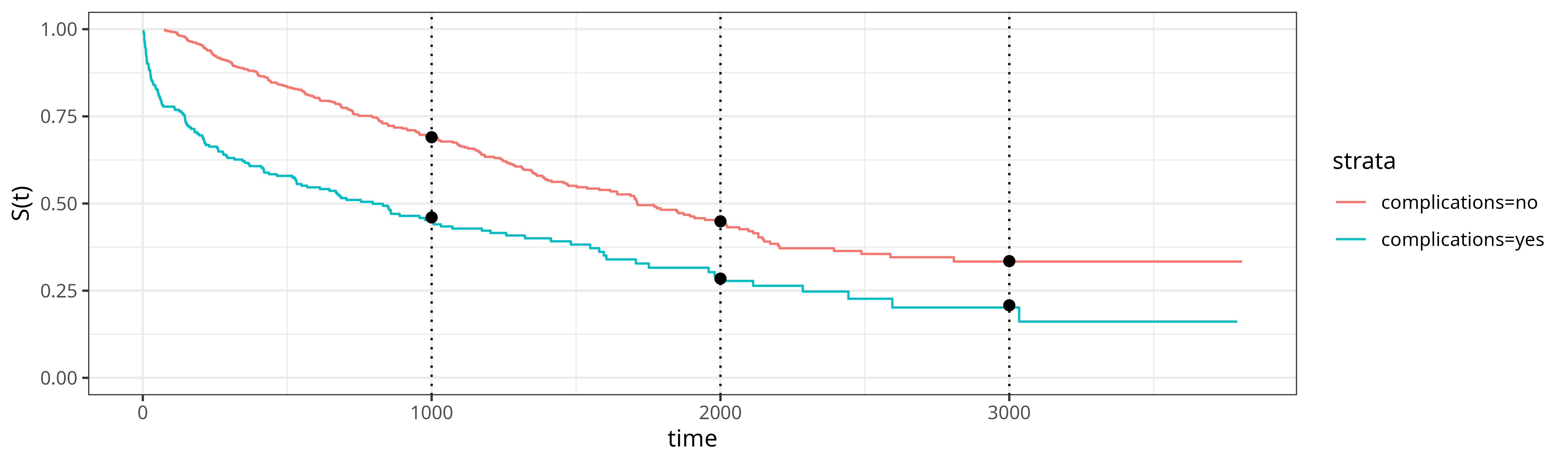
In a next step, we include complications as a predictor and specify \[ \hat{S}(\tau|\mathbf{x}_i) = \hat{\beta}_{\tau,0} + \hat{\beta}_{\tau,1} x_{i,1},\quad x_{i,1} = \mathbb{I}(\text{complications}_i = \text{"yes"}). \tag{17.7}\] We also repeat the analysis for each time-point \(\tau \in \{1000, 2000, 3000\}\) days separately. The results are shown in Figure 17.1, where the black dots indicate the survival probability predictions from the pseudo-value based approach and the solid lines are Kaplan-Meier estimates of the survival probability for comparison. Notably, the Kaplan-Meier estimates in the graphic have been obtained separately for each group (that is stratified by the complication variable) and the results indicate that the proportional hazards assumption does not hold for this example, as the shape of the survival function differs between the two groups (intuitively, patients with complications have a higher hazard in the first days after operation and therefore lower survival probability). The Kaplan-Meier estimates used for the calculation of the pseudo-values on the other hand were obtained by applying a univariate Kaplan-Meier estimator. Despite not stratifying the estimator when calculating the pseudo-values, the pseudo-value based approach still obtains correct estimates of the survival probabilities at the selected time points for both groups. This works even when the proportional hazards assumption is violated as the linear model is fit to each time-point separately and thus is able to learn different values of \(\hat{\beta}_{\tau,0}\) and \(\hat{\beta}_{\tau,1}\) for each \(\tau\).
Because we use the identity response function in the linear model, \(\hat{\beta}_{\tau,1}\) can be interpreted directly as the effect of complications on the survival probability at time \(\tau\). Here, \(\hat{\beta}_{1000,1}\approx -0.23\) and so the expected survival probability at time \(\tau = 1000\) for patients with complications is reduced by around 23 percentage points compared to patients without complications. In contrast, in a Cox model (Section 10.2) with linear predictor \(\eta_i = \beta_0 + \beta_1 x_{i,1}\), \(\beta_1\) can only be directly interpreted in terms of (log-)hazard ratios rather than survival probabilities (and under the proportional hazards assumption). Also note that the above results only hold for \(\tau = 1000\). At \(\tau = 2000\) days, \(\hat{\beta}_{2000,1} \approx -0.18\), and at \(\tau = 3000\) days, \(\hat{\beta}_{3000,1} \approx -0.13\), thus the average effect of complications depends on \(\tau\) and decreases over time (complications have a time-varying effect).
Besides the direct (time-varying) interpretation of the feature effects this might still feel overly complex given that similar results can be extracted from the stratified Kaplan-Meier analysis. However, once we add continuous features like age, Kaplan-Meier estimators are no longer applicable. Other models like Cox models assume proportional hazards and the estimated effects are expressed in terms of hazard ratios rather than survival probabilities.
Thus, in a final illustration, we add age to the model, such that
\[ \hat{S}(\tau|\mathbf{x}_i) = \hat{\beta}_{\tau,0} + \hat{\beta}_{\tau,1} x_{i,1} + \hat{\beta}_{\tau,2} x_{i,2},\quad x_{i,1} = \mathbb{I}(\text{complications}_i = \text{"yes"}), x_{i,2} = \text{age}_i \]
The resulting estimates are given in Table 17.2, where the effects of age and complications are given for each time-point \(\tau \in \{1000, 2000, 3000\}\) days separately.
| \(\tau\) | \(\hat{\beta}_{\tau,1}\) | \(\hat{\beta}_{\tau,2}\) |
|---|---|---|
| 1000 | -0.2205 | -0.0032 |
| 2000 | -0.1428 | -0.0070 |
| 3000 | -0.1050 | -0.0071 |
Conditional on \(\tau\), the interpretation is equivalent to a standard multiple linear regression model. For example, at \(\tau = 1000\) days, the effect of age is \(\hat{\beta}_{1000,2} \approx -0.0032\), which means that, given everything else being equal, the expected survival probability is reduced by ca 0.32 percentage points per additional year of age. Considering the change of the coefficients over time, one can conclude that the effect of complications decreases over time while the effect of age increases between 1000 and 2000 days and then appears to remain stable at around \(0.7\) percentage points per additional year.
17.2 Pseudo-values for RMST
An unbiased, univariate estimator for the restricted mean survival time (RMST; Equation (5.2)) can be obtained via \[ \text{RMST}(\tau) = \int_0^\tau S_{KM}(u) du, \] such that the calculated pseudo-values are given by \[ \tilde{\theta}_i(\tau) = n \widehat{\text{RMST}}(\tau) - (n-1)\widehat{\text{RMST}}^{-i}(\tau), \tag{17.8}\] where \(\tilde{\theta}_i(\tau)\) is now the pseudo-value of the restricted mean survival time at time \(\tau\) for observation \(i\).
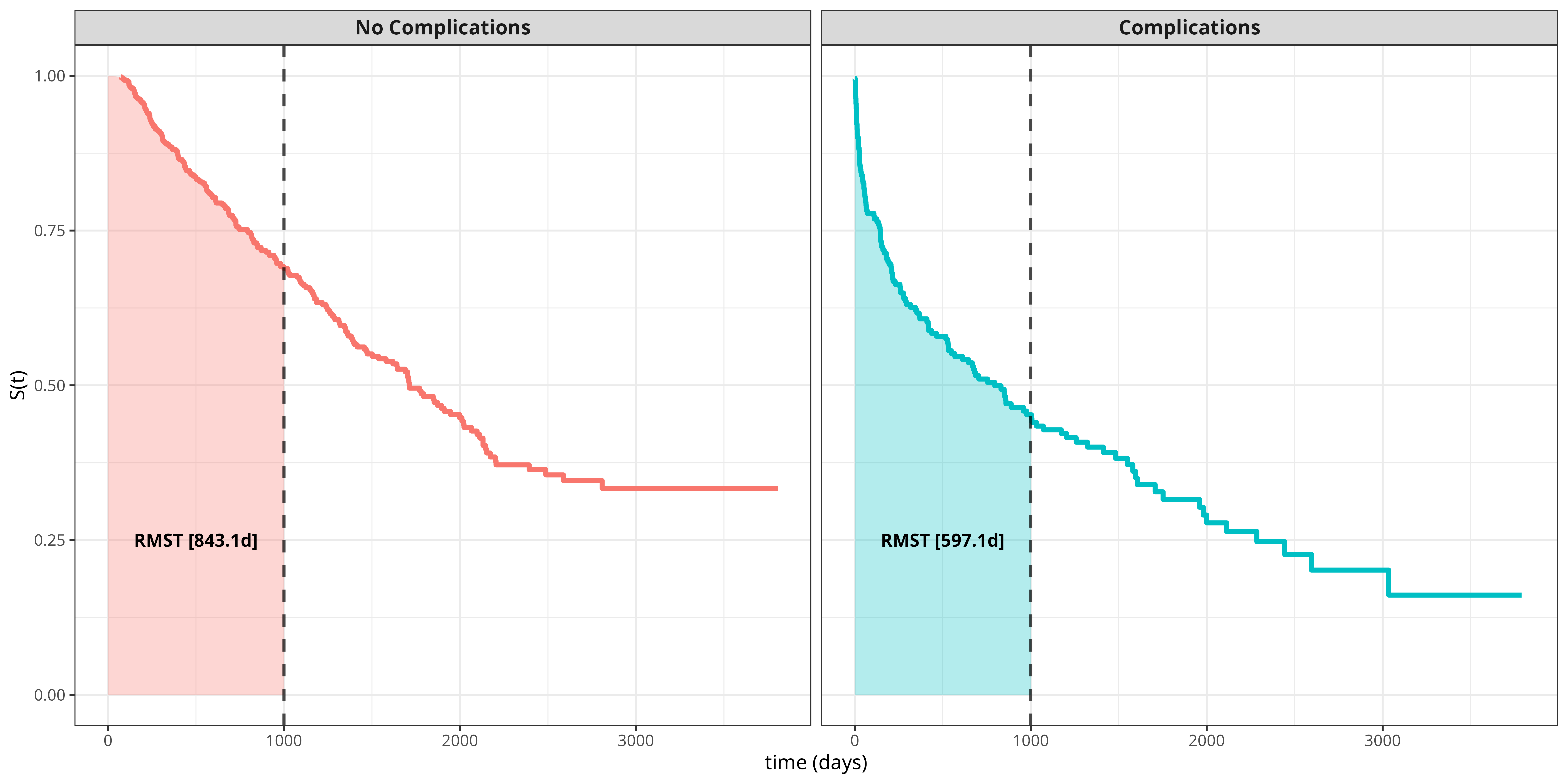
Continuing the tumor data example from Section 17.1, we are now interested in the RMST and how it depends on covariates. The general idea is illustrated in Figure Figure 17.2, which displays survival curves for each group (complications vs. no complications) with the RMST shown as the area under the curve up to \(\tau = 1000\) days. If one is interested in the difference between patients with and without complications, then the difference in RMSTs between the two groups can be calculated, which around \(246\) days in this example. Thus, within the first 1000 days after operation, patients with complications are expected to live 246 days less than patients without complications.
For a pseudo-value based analysis, we once again fit a linear model \[ \hat{\tilde{\theta}}_i(\tau) = \widehat{\text{RMST}}(\tau|\mathbf{x}_i) = \hat{\beta}_{\tau,0} + \hat{\beta}_{\tau,1} x_{i,1} \]
For time point \(\tau = 1000\) days, we obtain an estimate of \(\hat{\beta}_1 \approx -239\). Thus, the expected RMST for patients with complications is reduced by around 239 days, which is similar to the result obtained from the Kaplan-Meier analysis in Figure Figure 17.2. However, using pseudo-values from (17.8), we can directly extend the predictor, for example by including age: \[ \hat{\tilde{\theta}}_i(\tau) = \hat{\beta}_{\tau,0} + \hat{\beta}_{\tau,1} x_{i,1} + \hat{\beta}_{\tau,2} x_{i,2} \] where \(x_{i,1}\) as before and \(x_{i,2}\) is the age of subject \(i\). The respective estimates are \(\hat{\beta}_1 \approx -230\) and \(\hat{\beta}_2 \approx -3\), such that, given everything else being equal, the expected RMST is reduced by circa 3 days per year of age. The effect of complications, \(\hat{\beta}_1\), is slightly reduced when age is included and can be interpreted as the effect of complications on RMST adjusted for age.
17.3 Pseudo-values in Event-History Analysis
The pseudo-value approach can be extended to more complex event-history settings, including competing risks and multi-state models (Andersen and Pohar Perme (2010); Parner et al. (2023); Andersen et al. (2003)). The key idea remains the same: use univariate, non-parametric estimators of the quantity of interest to calculate pseudo-values, which can then be used as target variables in regression models.
17.3.1 Pseudo-values for Competing Risks
In the competing risks setting (Section 4.2), a quantity of particular interest is the cumulative incidence function (CIF) \(F_e(\tau)\) (4.9), which represents the probability of experiencing event type \(e\) before time \(\tau\). A suitable, univariate, unbiased estimator for the CIF is the Aalen-Johansen estimator. Pseudo-values for the CIF are thus given by \[ \theta_{i,e}(\tau) = nF_{AJ,e}(\tau) - (n-1)F_{AJ,e}^{-i}(\tau), \tag{17.9}\] where \(F_{AJ,e}^{-i}(\tau)\) is the Aalen-Johansen estimator of the CIF for event type \(e\) obtained by omitting the \(i\)-th observation from the data set.
Once calculated, these pseudo-values can once again be used as target variables in regression models to estimate the conditional CIF \(F_e(\tau | \mathbf{x}_i)\) via 17.3. This allows for direct interpretation of covariate effects on the cumulative incidence of a specific event type.
17.3.2 Pseudo-values for Multi-State Models
In multi-state settings (Section 4.3), pseudo-values are often used in order to estimate state occupation probabilities conditional on features. These represent the probability of being in state \(e\) at time \(\tau\). Non-parametric estimators for state occupation probabilities can be obtained via the Aalen-Johansen estimator for multi-state models (Section 4.3.4). The pseudo-values for state occupation probabilities are then defined as
\[ \tilde{\theta}_{i,e}(\tau) = nP_{AJ,e}(\tau) - (n-1)P_{AJ,e}^{-i}(\tau), \tag{17.10}\]
where \(P_{AJ,e}(\tau)\) is the Aalen-Johansen estimator of the state occupation probability for event type \(e\) at time \(\tau\), and \(P_{AJ,e}^{-i}(\tau)\) is the same estimator obtained by omitting the \(i\)-th observation.
These pseudo-values can be used to model conditional state occupation probabilities \(P_e(\tau | \mathbf{x}_i)\) using standard regression techniques. This approach is particularly flexible as it allows for modeling state occupation probabilities directly, without the need to specify and estimate all transition hazards (Andersen et al. (2003)).
17.4 Advantages and Limitations
Although the examples given in (Section 17.1) and (Section 17.2) are relatively simple, they illustrate the main advantages and limitations of the pseudo-value approach for machine learning based survival analysis:
On the plus side one can,
- estimate/predict various quantities of interest at selected time points \(\tau\), conditional on covariates, as long as an univariate, unbiased estimator of the quantity of interest is available,
- learn function \(f(\mathbf{x})\) in 17.3 using any regression machine or deep learning method for uncensored data without any additional modifications by using the pseudo-values as target variables,
- interpret the effects of features directly as effects on the quantity of interest \(\psi(\tau|\mathbf{x})\) (at least when the response function \(h\) in 17.3 is the identity function).
- when used in usual machine learning workflows, pseudo-values are calculated for the entire data set before splitting the data into training and test sets
- no survival specific metrics are needed for training and validation as pseudo-values can be considered uncensored data. However, since predictions (after application of the response function) reflect the quantity of interest, evaluation can also be performed using survival metrics in combination with the untransformed (censored data), for example when comparing the predictions with predictions from survival learners.
However, there are also some limitations:
- Pseudo-values can take on positive and negative values, therefore it is not guaranteed that the model predictions are within the range of the target. For example, survival probabilities should be within \([0,1]\), which can only be insured if the response function \(h\) is chosen suitably. In context of statistical modeling, generalized estimating equations (Hardin and Hilbe (2012)) with suitable link functions can be used to ensure that the predictions are within the range of the target (standard GLMs are not suitable as the pseudo-values are not necessarily in the range of the target space). In machine learning, similar approaches can be used, for example by clipping the predictions to the range of the target or using suitable transformations/activation functions. However, even without transformation, predictions will often be within the desired range, especially if \(\tau\) is not at the edge of the follow-up period (where the survival probability is close to 0 or 1) and if \(\mathbf{x}\) is not an outlier in the feature space.
- Pseudo-values are technically not independent (all observations are used to calculate \(\hat{\psi}(\tau)\) and most to calculate \(\hat{\psi}^{-i}(\tau)\)); this does not affect the estimation of \(f(\mathbf{x})\) too much, but robust variance estimation is preferred in context of statistical inference, for example using generalized estimating equations with robust (sandwich) variance estimation.
- Interpretation of feature effects is hindered to some extent by being time dependent; this can however also be viewed as an advantage, as the approach does not make strict assumptions like proportional hazards or accelerated failure time assumptions, which can be violated in practice.
- Calculating pseudo-values can be computationally expensive if predictions are needed at many time points \(\tau\) and for many observations \(i\), as the univariate estimator \(\psi(\tau)\) has to be calculated \(n + 1\) times per time point. However, for specific use cases efficient implementations based on infinitesimal jack-knife and other methods have been suggested in the literature and implemented in standard software packages (Parner et al. (2023), Bouaziz (2023)).