5 Survival Task
This page is a work in progress and minor changes will be made over time.
The preceding chapters have focused on understanding survival data. This final chapter turns to the prediction tasks themselves.
Recall from Section 2.1 that a general survival prediction problem is one in which:
- a survival dataset, \(\mathcal{D}\), is split for training, \(\mathcal{D}_{train}\), and testing, \(\mathcal{D}_{test}\);
- a survival model is fit on \(\mathcal{D}_{train}\); and
- the model predicts a representation of the unknown true survival time, \(Y\), given \(\mathcal{D}_{test}\).
The process of model fitting is model-dependent and ranges from non-parametric methods to machine learning approaches; these are discussed in Part III. Discussing the typical ‘representations of \(Y\)’ will be the focus of this chapter.
In general there are four common prediction types or prediction problems which codify different representations of \(Y\), these are:
- Survival distributions;
- Time-to-event;
- Relative risks;
- Prognostic index.
The first of these is considered probabilistic as it predicts the probability of an event occurring over time. The second is deterministic as the prediction is a single point prediction. The final two do not directly predict the event of interest but instead provide different interpretations that both relate to the risk of the event. The relative risks and time-to-event prediction types can both be derived from a survival distribution prediction, and the prognostic index is often used as an interim step before making a probabilistic prediction (see ?sec-surv-models-crank); so all of these prediction types are closely related.
It is vital to clearly separate which prediction problem you are working with, as they are not directly compatible with one another. For example, it is not meaningful to compare a relative risk prediction from one model to a survival distribution prediction of another. Moreover, prediction types may look similar but have very different implications, for example if one erroneously interprets a survival time as a relative risk then they could assume an individual has a worse outcome than they do as longer survival times imply lower risk.
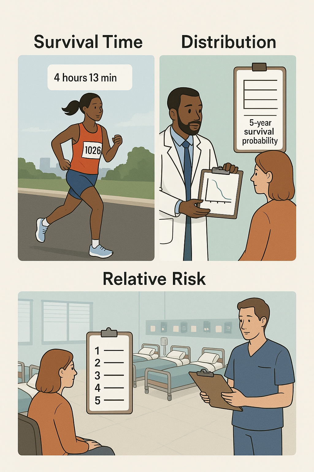
Each prediction type has its own particular advantages and disadvantages and should be used appropriately. For example, survival times are not advised in domains where over-confidence can be detrimental, but can be used when making less-critical predictions, such as a marathon runner’s finish time (Figure 5.1, top-left), which is a survival analysis problem as many people do not finish. Whilst clinicians will usually not present a probability distribution to a patient (Figure 5.1, top-right), it is common to relay information such as ‘5-year survival probability’, which is read from a predicted survival distribution. Finally, relative risk predictions are often used for triage and resource allocation, such as assigning patients to particular wards or beds (Figure 5.1, bottom).
Whilst one prediction type is necessary to define a model’s output, it is often the case that an algorithm might use another prediction type as an interim prediction. This chaining of predictions is called ‘composition’ as two components are composed to create a final prediction, this is commonly the case for distribution predictions. It is also possible to convert prediction types between one another. Table 5.1 highlights how distribution and survival time predictions can be transformed to most other forms and how all forms can be transformed to a relative risk prediction. These transformations will be discussed in more detail in the rest of this chapter.
Throughout this chapter let \(\mathcal{X}\subseteq \mathbb{R}^{n \times p}\) be a set representing covariates. Note that the type of censoring in the data is part of the estimation problem and does not affect the prediction types, hence this chapter does not differentiate between right, left, or interval censoring. The focus is primarily on the single-event setting, a brief section on other settings is included at the end of the chapter.
| Distribution | Risk | Time | PI | |
|---|---|---|---|---|
| Distribution, \(\hat{S}\) | \(\hat{S}\) | \(\sum_t \hat{H}(t)\) | \(\operatorname{RMST}(\tau)\) | NA |
| Risk, \(\hat{r}\) | \(\Phi(\hat{r})\) | \(\hat{r}\) | NA | NA |
| Time, \(\hat{y}\) | \(\operatorname{Distr}(\hat{y}, \sigma)\) | \(-\hat{y}\) | \(\hat{y}\) | NA |
| PI, \(\hat{\eta}\) | \(\phi(\hat{\eta}, \hat{y})\) | \(\hat{\eta}\) or \(-\hat{\eta}\) | NA | \(\hat{\eta}\) |
5.1 Predicting Distributions
Predicting a survival distribution means predicting the probability of an individual surviving over time from \(0\) to \(\infty\). Ideally one would make predictions over the continuous \(\mathbb{R}_{\geq 0}\), however, in practice it is more common for predictions to be made over \(\mathbb{N}_0\). This is due to the majority of models using discrete non-parametric estimators to create a distribution prediction. Distributional prediction can, in theory, target any of the distribution defining functions introduced in Section 3.1, but predicting \(S(t)\) and/or \(h(t)\) is most common. This is a probabilistic survival task as uncertainty is explicit in the prediction. Mathematically, the task is defined by \(g: \mathcal{X}\rightarrow \mathcal{S}\) where \(\mathcal{S}\subseteq \operatorname{Distr}(\mathbb{R}_{\geq 0})\) is a set of distributions on \(\mathbb{R}_{\geq 0}\).
Practically, especially in healthcare, survival distribution predictions are often used to estimate ‘\(\tau\)-year survival probabilities’, which is the probability of survival at a given point in time. Therefore a clinician is not likely to display a survival curve to a patient, but may use their individual features to compute probabilities of survival at key time-points (often, 5, 10 years) – an example of this in use is the PREDICT breast cancer tool (Candido dos Reis et al. 2017). In other contexts, such as engineering, survival distributions might be used to establish thresholds for replacing components. For example, one could use a survival model to estimate the reliability of a plane engine over time, a threshold could be set such that the engine will be replaced when \(\hat{S}(t) < 0.6\).
Predicting \(\tau\)-year survival probabilities is often confused with a classification problem, which make probabilities for one or more events occurring at a fixed point in time. However, a classification model would be unable to use any observations that were censored before the time of interest and discarding these observations would bias any results (Loh et al. 2025).
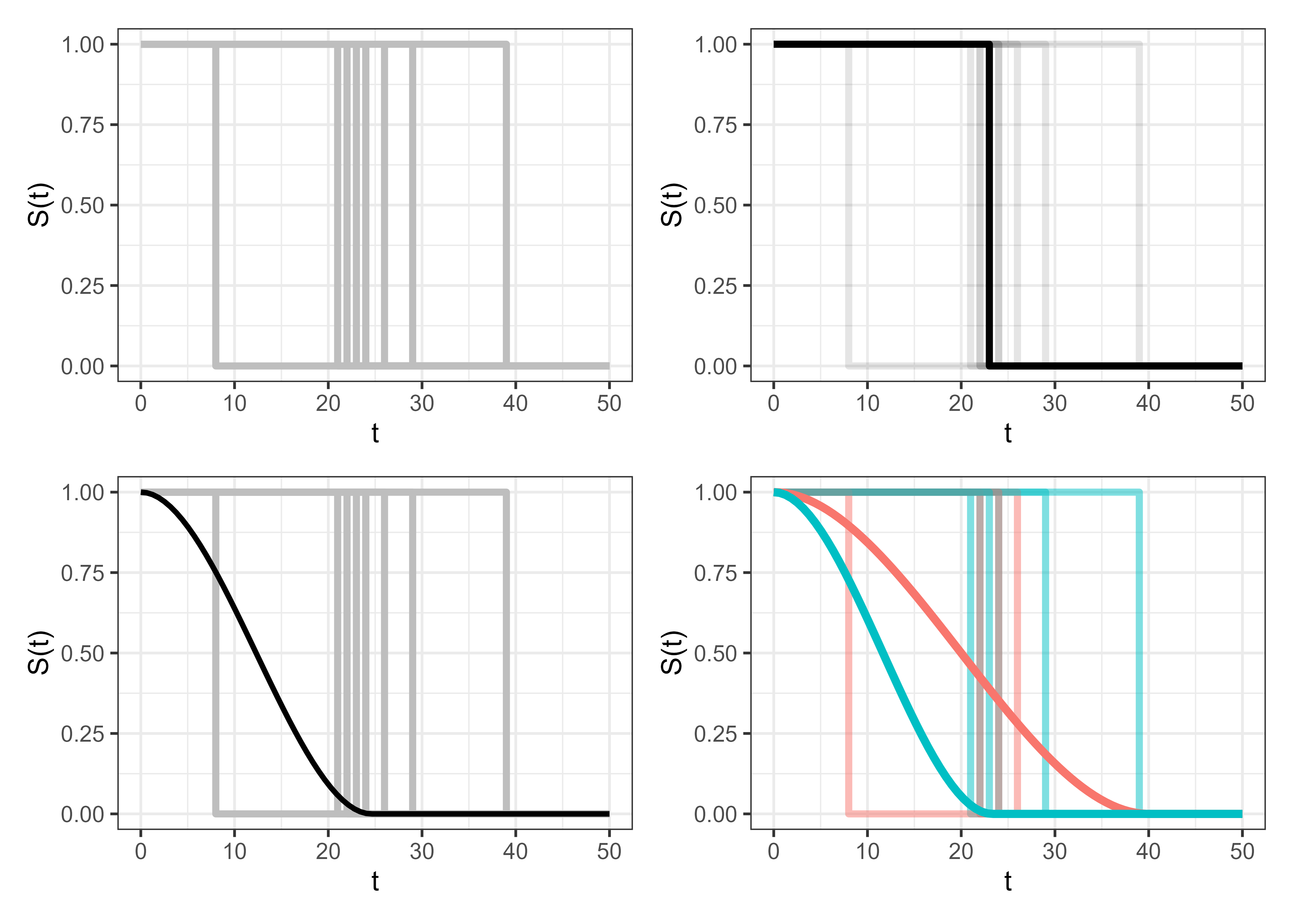
Another potential source of confusion can arise when trying to figure out what it actually means to predict a distribution that represents a single event occurring for a single observation. In reality, something either does or does not happen at a point in time, so what does it really mean to predict a distribution around this event? To make this clear, Figure 5.2 visualizes what the survival task aims to achieve. The top-left image shows the real-world distribution when an event occurs, this is a heaviside function where the survival probability drops immediately from \(1\) to \(0\) when the event occurs; the top-right image highlights this curve for a single event. The bottom-left shows what we aim to achieve, which is a survival curve prediction that accurately captures the average survival distribution across all of these events. Finally, the bottom-right curve shows the same events split according to a single, binary covariate with one prediction per covariate value. In a machine learning task, this is essentially repeated for every possible combination of covariates.
5.2 Predicting Risks
Predicting risks is defined as predicting a continuous rank for an individual’s relative risk of experiencing the event. Therefore this might also be known as a ‘ranking’ problem or predicting ‘continuous rankings’. In machine learning terms, this task is the problem of estimating, \(g: \mathcal{X}\rightarrow \mathbb{R}\).
Interpretation of these rankings is more complex than might be imagined as the meaning differs between models, parametrizations, and even software implementations. To be consistent, in this book a larger risk value always corresponds to a higher risk of an event and lower values corresponding to lower risk.
A potential confusion that should be avoided is conflating this risk prediction with a prediction of absolute risk. Risk predictions are specifically relative risks, which means the risks are only comparable to other observations within the same sample. For example, given three subjects, \(\{i,j,k\}\), a risk prediction may be \(\{0.5, 10, 0.1\}\) respectively. From these predictions, two primary types of conclusion can be drawn.
- Conclusions comparing subjects:
- The corresponding ranks for \(i,j,k\) are \(2,3,1\);
- \(k\) is at the least risk and \(j\) is at the highest risk;
- The risk of \(i\) is slightly higher than that of \(k\) but \(j\)’s risk is considerably higher than both the others.
- Conclusions comparing risk groups:
- Thresholding risks at \(0.4\) means \(k\) is at a low-risk but \(i\) and \(j\) are high-risk.
- Thresholding risks at \(1.0\) means \(i\) and \(k\) are low-risk but \(j\) is high-risk.
Whilst many important conclusions can be drawn from these predictions, the values themselves have no meaning when not compared to other individuals. Similarly, the values have no meanings across research, even if observation \(k\) is at low-risk according to this sample, it may be high risk compared to another. Finally, as with relative risks in other domains, differences in relative risk should be interpreted with care. In the example above, \(j\)’s relative risk is 100 times that of \(k\), but if \(k\)’s overall probability of experiencing the event is \(0.0001\), then \(j\)’s overall probability of experiencing the event is still only \(0.01\).
5.2.1 Distributions and risks
In general it is not possible to easily convert a risk prediction to a distribution. However, this may be possible if the risk prediction corresponds to a particular model form. This is discussed further in Section 5.4.
More common is transformation from a distribution to a risk. Theoretically the simplest way to do so would be to take the mean or median of the distribution, however as will be discussed in detail in Section 5.3 this is practically difficult. Instead, a stable approach is to use the ‘ensemble’ or ‘expected mortality’ to create a measure of risk (Ishwaran et al. 2008). The expected mortality is defined by
\[ \sum_t -\log(\hat{S}_i(t)) = \sum_t \hat{H}_i(t) \]
and is closely related to the calibration measure defined in Section 7.1.2. This represents the expected number of events for individuals with similar characteristics to \(i\). This is a measure of risk as a larger value indicates that among individuals with a similar profile, there is expected to be a larger number of events and therefore have greater risk than those with smaller ensemble mortality. For example, say for an individual, \(i\), we have: \((t, \hat{S}_i(t)) = (0, 1), (1, 0.8), (2, 0.4), (3, 0.15)\) then, \((t, \hat{H}_i(t)) = (0, 0), (1, 0.10), (2, 0.40), (3, 0.82)\), then their relative risk prediction is \(\sum_t \hat{H}_i(t) = 0 + 0.10 + 0.4 + 0.82 = 1.32\).
5.3 Predicting Survival Times
Predicting a time-to-event is the problem of estimating when an individual will experience an event. Mathematically, the problem is the task of estimating \(g: \mathcal{X}\rightarrow \mathbb{R}_{>0}\), that is, predicting a single value over \([0,\infty]\).
For practical purposes, the expected time-to-event would be the ideal prediction type as it is easy to interpret and communicate. However, evaluation of these predictions is tricky. Take the following example. Say someone is censored at \(\tau=5\), there is no way to know if they would have experienced the event at \(\tau=6\) or \(\tau=600\), all that can be known is that the model correctly identified they did not experience the event before \(\tau=6\). Furthermore, if the model had predicted \(\tau=3\), metrics such as mean absolute error would be misleading, as an MAE of \(5 - 3 = 2\) would make the model seem artificially better than it was, if the event actually occurred at \(\tau=600\). Therefore, when an observation is censored, the best one can do is evaluate a classification task: did the model predict that the event did not occur before the censoring time. As this is not the task of interest, one is left to evaluate uncensored observations only, which can introduce bias to the evaluation. Given this complexity, the time-to-event point prediction is rare in practice.
5.3.1 Times and risks
Converting a time-to-event prediction to a risk prediction is trivial as the former is a special case of the latter. An individual with a longer survival time will have a lower overall risk: if \(\hat{y}_i,\hat{y}_j\) and \(\hat{r}_i,\hat{r}_j\) are survival time and ranking predictions for subjects \(i\) and \(j\) respectively, then \(\hat{y}_i > \hat{y}_j \Rightarrow \hat{r}_i < \hat{r}_j\). It is not possible to make the transformation in the opposite direction without making significant assumptions as risk predictions are usually abstract quantities that rarely map to realistic survival times.
5.3.2 Times and distributions
Moving from a survival time to a distribution prediction is rare given the reasons outlined above. Theoretically one could make a prediction for the expected survival time, \(\hat{y}\) and then assume a particular distributional form. For example, one could assume \(\operatorname{TruncatedNormal}(\hat{y}, \sigma, a=0, b=\infty)\) where \(\hat{y}\) is the predicted expected survival time, \(\sigma\) is a parameter representing variance to be estimated or assumed, and \(\{a, b\}\) is the distribution support. This method clearly has drawbacks given the number of required assumptions and as such is not commonly seen in practice.
In the other direction, it is common to to reduce a distribution prediction to a survival time prediction by attempting to compute the mean or median of the distribution. When there is no censoring, one can calculate the expectation from the predicted survival function using the ‘Darth Vader rule’ (Muldowney et al. 2012):
\[ \mathbb{E}[Y] = \int^\infty_0 S_Y(y) \ \text{d}y \tag{5.1}\]
However, this rule is rarely usable in practice as censoring results in estimated survival distributions being ‘improper’. A valid probability distribution for a random variable \(Y\) satisfies: \(\int f_Y = 1\), \(S_Y(0) = 1\) and \(S_Y(\infty) = 0\). This last condition is often violated in survival distribution predictions, which often use semi-parametric methodology (?sec-surv-models-crank), resulting in improper distributions. Recall from Section 3.5.2.1 that the Kaplan-Meier estimator is defined as:
\[ \hat{S}_{KM}(\tau) = \prod_{k:t_{(k)} \leq \tau}\left(1-\frac{d_{t_{(k)}}}{n_{t_{(k)}}}\right) \]
This only reaches zero if every individual at risk at the last observed time-point experiences the event: \(d_{t_{(k)}} = n_{t_{(k)}}\). In practice, due to administrative censoring, there will almost always be censoring at the final time-point. As a result, \(d_{t_{(k)}} < n_{t_{(k)}}\) and \(\hat{S}(\infty) > 0\). Heuristics have been proposed to address this including linear extrapolation to zero, or dropping the curve to zero at the final time-point, however these can introduce significant bias in the estimated survival time (Han and Jung 2022; Sonabend et al. 2022). Another possibility is to instead report the median survival time, but this is only defined if the survival curves drop below \(0.5\) within the observed period, which is not guaranteed (Haider et al. 2020).
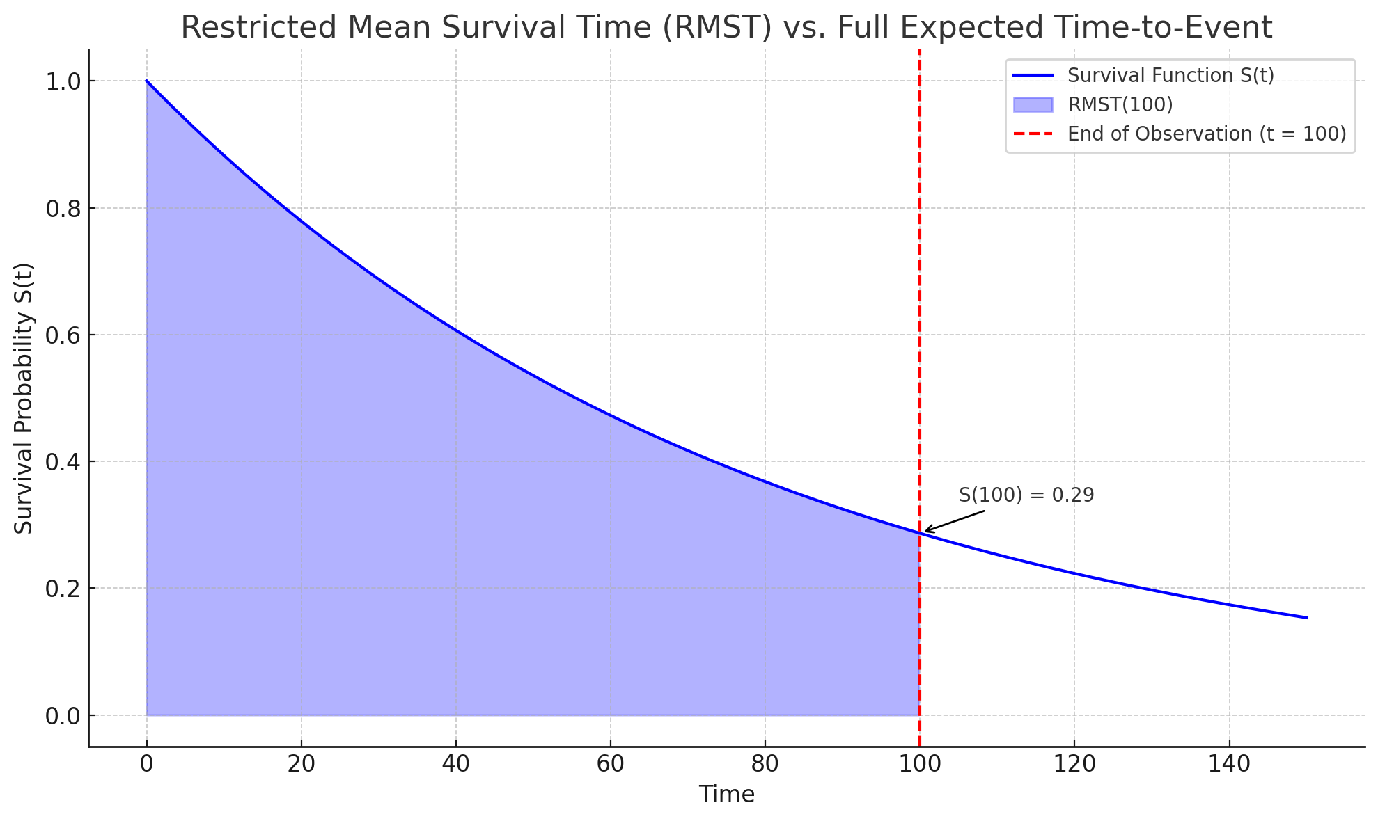
One alternative is to estimate the restricted mean survival time (RMST) (Han and Jung 2022; Andersen et al. 2004). In contrast to 5.1, which integrates the survival curve over the entire time axis, the RMST places an upper-bound on the integral:
\[ \operatorname{RMST}(\tau) = \int^\tau_0 S_Y(y) \ \text{d}y \tag{5.2}\]
Clearly then \(\operatorname{RMST}(\infty) = \mathbb{E}[Y]\) by 5.1. Whereas 5.1 represents the average survival over \([0,\infty)\), 5.2 represents the average survival time up to \(\tau\). Equivalently, the RMST is the average amount of time each individual spends without experiencing the event up to \(\tau\). The RMST treats all events happening after \(\tau\) as if they happened at \(\tau\). Hence, it is a truncated expectation, estimating: \(\mathbb{E}[\min(Y, \tau)]\)
For example, say individuals are observed over times \([0,100]\) and administrative censoring is present in the data, then \(\hat{S}(\tau)\) is unknown for \(\tau > 100\) and \(\mathbb{E}[Y]\) cannot be reliably computed. However, one can compute \(\operatorname{RMST}(100)\) which provides an interpretable lower bound for the mean survival time: \(\operatorname{RMST}(100) \leq \mathbb{E}[Y]\). This avoids assumptions beyond \(\tau=100\) and offers an interpretable prediction: “the average survival time is at least \(\operatorname{RMST}(100)\)” (Figure 5.3). The RMST avoids the pitfalls of computing the mean and median by remaining valid even when the predicted distribution is improper, provided that \(\tau\) is chosen within the range of observed follow-up times.
As a worked example, say for an individual, \(i\), we have: \((t, \hat{S}_i(t)) = (0, 1), (1, 0.8), (2, 0.4), (3, 0.15)\). Using a Riemann sum approximation, \(\operatorname{RMST}(3) \approx 1 + 0.8 + 0.4 = 2.2\) and \(\operatorname{RMST}(4) \approx 1 + 0.8 + 0.4 + 0.15 = 2.35\). \(\operatorname{RMST}(3)\) reflects the expected time without experiencing the event up to \(\tau=3\), which means treating all observations as if the event occurred at \(\tau=3\) (unless it occurred sooner). \(\operatorname{RMST}(4)\) incorporates one more unit of follow-up, including the fourth survival probability in this case. In this way, the \(\operatorname{RMST}(\tau)\) summarizes the average survival experience up until \(\tau\), smaller values of \(\tau\) emphasize near-term survival whereas larger values approach the full mean survival time (if estimable). The actual choice of \(\tau\) varies by the use-case.
5.4 Prognostic Index Predictions
In medical terminology (often used in survival analysis), a prognostic index is a tool that predicts outcomes based on risk factors. Given covariates, \(\mathbf{X}\in \mathbb{R}^{n \times p}\), and coefficients, \(\boldsymbol{\beta}\in \mathbb{R}^p\), the linear predictor is defined as \(\boldsymbol{\eta}:= \mathbf{X}\boldsymbol{\beta}\). Applying some function \(g\), which could simply be the identity function \(g(x) = x\), yields a prognostic index, \(g(\boldsymbol{\eta})\). A prognostic index can serve several purposes, including:
- Scaling or normalization: simple functions to scale the linear predictor can better support interpretation and visualisation;
- Ensuring meaningful results: for example the Cox PH model (Chapter 10) applies the transformation \(g(\boldsymbol{\eta}) = \exp(\boldsymbol{\eta})\), which guarantees positivity of hazards as well as making the covariates multiplicative;
- Aiding in interpretability: in some cases this could simply be \(g(\boldsymbol{\eta}) = -\boldsymbol{\eta}\) to ensure the ‘higher value implies higher risk’ interpretation.
5.4.1 Prognostic index, risks, and times
A prognostic index is a special case of the survival ranking task, assuming that there is a one-to-one mapping between the prediction and expected survival times. For example, one could define \(g(\boldsymbol{\eta}) = 1 \text{ if } \eta < \text{5 or } 0 \text{ otherwise }\) however this would prevent the prognostic index being used as a ranking method and it would defeat the point of a prognostic index.
As with a risk prediction, there is no general relationship between the prognostic index and survival time. However, there are cases where there may be a clear relationship between the two. For example, one can theoretically estimate a survival time from the linear predictor used in an accelerated failure time model (?sec-surv-models).
5.4.2 Prognostic index and distributions
A general prognostic index cannot be generated from a distribution, however the reverse transformation is very common in survival models. The vast majority of survival models are composed from a group-wise survival time estimate and an estimation of an individual’s prognostic index. This will be seen in detail in future chapters (particularly in Chapter 13 and Chapter 14) but in general it is very common for models to assume data follows either proportional hazards or accelerated failure time (Chapter 10). In this case models are formed of two components:
- A ‘simple’ model that can estimate the baseline hazard, \(\hat{h}_0\), or baseline survival function, \(\hat{S}_0\). Discussed further in Chapter 10, these are group-wise estimates that apply to the entire sample.
- A sophisticated algorithm that estimates the individual linear prediction, \(\hat{\eta}\).
These are composed as either:
- \(\hat{h}_0(t)\exp(\hat{\eta})\) if proportional hazards is assumed; or
- \(\hat{h}_0(\exp(-\hat{\eta})t)\exp(-\hat{\eta})\) for accelerated failure time models.
5.5 Beyond single-event
In Chapter 4, competing risks and multi-state models were introduced with a focus on estimating probability distributions.
In the competing risks setting, ‘survival time’ is ill-defined, it is ambiguous whether this refers to the time until a specific event or until any event takes place. In principle, one could apply the RMSE approach to the all-cause survival function, though this is uncommon in practice. Analogous to the single-event setting, a cause-specific prognostic index can be derived from a cause-specific cumulative incidence function, and vice versa. One might also consider transformations based on all-cause risk, but again such approaches are rarely used in applied settings.
In multi-state models, the primary prediction targets are transition probabilities between states over time (Section 4.3). Unlike standard survival settings, there is no single notion of a ‘survival time’. Instead, one can estimate the sojourn time, which is the expected time spent in a given state, using the estimated transition probabilities. This is particularly well-defined in Markov or semi-Markov models, where sojourn times follow from standard stochastic process theory. These derivations are beyond the scope of this book; for further detail, see for example (Ibe 2013).