18 Partition based reductions
This page is a work in progress and major changes will be made over time.
In contrast to the previously introduced reductions that focus on the estimation of a specific quantity of interest at one or few time points, partition-based reduction aim to estimate the entire distribution of the event times (similar to Cox models and other survival learners). The general idea is to partition the time axis into \(J\) intervals \((a_0,a_1],\ldots,(a_{J-1},a_J]\) and estimate a discrete or continuous hazard rate for each interval.
For illustration, consider the partitioning of the follow up in Figure Figure 18.1. Note that the intervals do not necessarily have to be equidistant. The \(j\)th interval is given by \(I_j:=(a_{j-1},a_j]\). Let further \(J_i\) the index of the interval in which observed time \(t_i\) of subject \(i\) falls, that is \(t_i \in I_{J_i} = (a_{J_i-1},a_{J_i}]\).
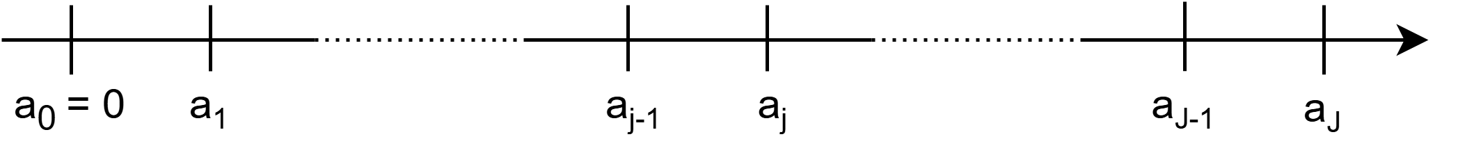
Formally, define the partitioning of the follow-up via the set of interval boundary points \(a_j\) for \(j=0,\ldots,J\) as
\[\mathcal{A} = \{a_0, \ldots, a_J\}, \quad a_0 < a_1 < \ldots < a_J \tag{18.1}\]
This partitioning is used to create a transformed data set. Using this transformed data, standard regression or classification methods can be used in order to estimate (discrete) hazards in each interval. Section 18.1 introduces the required data transformation formally. Section 18.2, Section 18.3 and Section 18.4 introduce specific reductions based on this data transformation, provide theoretical justification why models applied to such transformed data are valid approaches for estimation in time-to-event analysis and provide illustrative examples for such models. Section 18.5 discusses computational aspects and modeling choices (related to the choice of interval boundaries \(a_j\)).
18.1 Data Transformation
In order to apply the reduction techniques introduced in the upcoming sections, standard time-to-event data needs to be transformed into a specific format. The transformation is based on the partitioning of the follow-up as illustrated in Figure Figure 18.1 and boundaries as defined in 18.1. The new data set contains \(J_i\) rows for each subject \(i\), that is one row for each interval in which subject \(i\) was at risk of experiencing an event.
For each subject \(i\), we record the the subject’s interval-specific event indicator \[\delta_{ij} = \begin{cases} 1, & t_i \in (a_{j-1}, a_j] \text{ and } \delta_i = 1 \\ 0, & \text{ else } \end{cases},\quad j=1,\ldots,J_i, \tag{18.2}\]
the time at risk in interval \(j\) \[t_{ij} = \begin{cases} a_j - a_{j-1}, & \text{ if } t_i > a_j \\ t_i - a_{j-1}, & \text{ if } t_i \in (a_{J_i-1}, a_{J_i}]\\ \end{cases},\quad j=1,\ldots,J_i, \tag{18.3}\]
as well as some representation of the time in interval \(j\), for example the interval midpoint or endpoint \[t_j = a_j \tag{18.4}\]
and the subject’s (potentially time-dependent)features \[\mathbf{x}_{ij} \tag{18.5}\] with \(\mathbf{x}_{ij} = \mathbf{x}_{i}\) for all \(j\), if the features are constant over time.
Thus, given the partition \(\mathcal{A}\), the standard time-to-event data \(\mathcal{D}= \{(t_i, \delta_i, \mathbf{x}_i)\}_{i=1,\ldots,n}\) is transformed to data \[\mathcal{D}_{\mathcal{A}} = \{(i, j, \delta_{ij}, t_{ij}, t_j, \mathbf{x}_{ij})\}_{i=1,\ldots,n;\ j=1,\ldots,J_i}, \tag{18.6}\] where \(i\) and \(j\) indices are usually only used for “book-keeping” purposes but are not used in modeling later on.
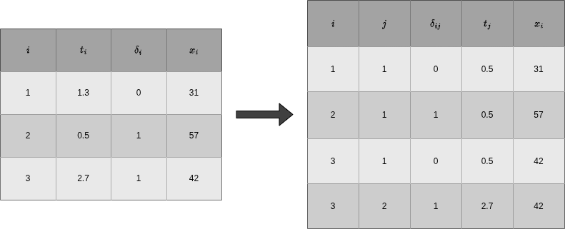
The data transformation procedure described above is illustrated in Figure Figure 18.2 for hypothetical data. The left hand side of Figure Figure 18.2 shows data in standard time-to-event format with one row per subject \(i=1,\ldots,3\) and \(\mathcal{D} = \{(1.3, 0, 31), (0.5, 1, 57), (2.7, 1, 42)\}\). For the transformation, we choose (arbitrary) interval boundaries \(\mathcal{A} = \{1, 1.5, 3\}\), which gives intervals \((0,1], (1,1.5], (1.5,3]\). The right-hand side of Figure Figure 18.2 shows the transformed data \(\mathcal{D}_{\mathcal{A}}\), where the first three columns keep track of subject and interval information and the other columns are the interval-specific event indicator, time at risk in the respective interval,representation of time and (time-dependent) features as defined in Equations 18.2, 18.3, 18.4 and 18.5, respectively.
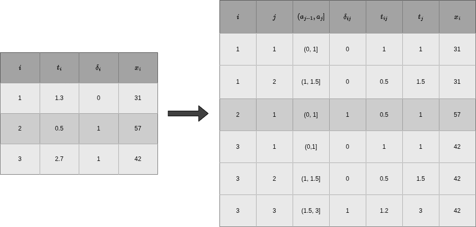
Note that \(\delta_{ij}=0\) for all intervals except the last of subject \(i\), where \(\delta_{iJ_i} = \delta_i\), so either 0 or 1. Thus the total number of events is the same in both the original and transformed data. In general, both data sets contain the same time-to-event information as the original data since, given the interval boundaries \(\mathcal{A}\), the variables \(\delta_{ij}\) and \(t_{ij}\) are deterministic functions of the original data.
18.2 Discrete Time Survival Analysis
Consider the partitioning of the follow-up 18.1 and assume we are only interested in whether the event occured within an interval rather than the exact event time. Using the notation from Section 3.1.2, the likelihood contribution of the \(i\)th observation is given by \(P(Y_i \in (a_{J_i-1}, a_{J_i}]) = P(\tilde{Y}_i = J_i)\) for subjects who experienced an event (\(\delta_i = 1\)) and \(P(Y_i > a_{J_i}) = P(\tilde{Y}_i > J_i)\) for subjects who were censored (\(\delta_i = 0\)).
Thus, using definitions 3.7 and 3.8, the likelihood contribution of subject \(i\) is given by \[\begin{aligned}L_i & = P(Y_i \in (a_{J_i-1}, a_{J_i}])^{\delta_i} P(Y_i > a_{J_i})^{1-\delta_i}\\ & = \left[S^d(J_i-1)h^d(J_i)\right]^{\delta_i} \left[S^d(J_i)\right]^{1-\delta_i}\\ & = \left[\left(\prod_{j=1}^{J_i-1} (1-h^d(j))\right)h^d(J_i)\right]^{\delta_i} \left[\prod_{j=1}^{J_i} (1-h^d(j))\right]^{1-\delta_i}, \end{aligned} \tag{18.7}\]
Now recall from Equation 18.2 the definition of the interval-specific event indicators \(\delta_{ij}\), which always take value 0, except for the last interval, where \(\delta_{iJ_i} = \delta_i\). Thus, the first part of 18.7 can be written as \(\prod_{j=1}^{J_i}(1-h^d(j))^{1-\delta_{ij}}h^d(j)^{\delta_{ij}}\) and the second part as \(\prod_{j=1}^{J_i}(1-h^d(j))^{1-\delta_{ij}}\). It follows, that the likelihood 18.7 can be written as \[\begin{aligned} L_i & = \left[\prod_{j=1}^{J_i} (1-h^d(j))^{1-\delta_{ij}}h^d(j)^{\delta_{ij}}\right]^{\delta_i} \left[\prod_{j=1}^{J_i} (1-h^d(j))^{1-\delta_{ij}}\right]^{1-\delta_i}\\ & = \prod_{j=1}^{J_i} (1-h^d(j))^{1-\delta_{ij}}h^d(j)^{\delta_{ij}}, \end{aligned} \tag{18.8}\] where the last equality follows from \(\delta_{ij}=0\ \forall j=1,\ldots,J_i\), if \(\delta_i = 0\) and thus \(\prod{1-h^d(j)}^{1-\delta_{ij}}h^d(j)^{\delta_{ij}} = \prod{1-h^d(j)}^{1-\delta_{ij}}\).
The importance of this result may not be immediately apparent, but recall that if \(Z \sim Bernoulli(\pi)\), where \(\pi = P(Z = 1)\), then likelihood contribution of \(Z\) is given by \(P(Z = z) = \pi^z (1-\pi)^{1-z}\). We therefore recognize that the likelihood contribution 18.8 can also be obtained by assuming that the interval-specific event indicators \(\delta_{ij}\) are realizations of random variables \(\Delta_{ij} \stackrel{iid}{\sim} Bernoulli(\pi_j = h^d(j))\). Thus \[\begin{aligned} \pi_j & = P(\Delta_{ij} = 1|t_j)\\ & = P(Y_i \in (a_{j-1}, a_j] | Y_i > a_{j-1}) = h^d(j) \end{aligned} \tag{18.9}\] Note that in 18.9, \(\Delta_{ij} =1\) is equivalent to \(Y_i \in (a_{j-1}, a_j]\), while the conditioning on \(Y_i > a_{j-1}\) is implicit in the definition of \(\delta_{ij}\) in 18.2.
This implies that we can estimate the discrete time hazards \(h^d(j)\) for each interval \(j\) by fitting any binary classifcation model to the transformed data set \[\mathcal{D}_{\mathcal{A}} = \{(\delta_{ij}, t_{j})\}_{i=1,\ldots,n;\quad j=1,\ldots,J_i}, \tag{18.10}\] where \(\delta_{ij}\) are the targets and \(t_{j}\), some representation of time in interval \(j\) (for example \(t_j = j\) or \(t_j = a_{j}\)), enters the estimation as a feature and is needed in order to estimate different hazards/probabilities in different intervals.
In the presence of features \(\mathbf{x}_{i}\) we assume \(\Delta_{ij}| \mathbf{x}_{i}, t_j \stackrel{iid}{\sim} Ber(\pi_{ij})\), where \(\pi_{ij} = P(\Delta_{ij} = 1| \mathbf{x}_{i}, t_j) = h^d(j|\mathbf{x}_{i})\) is the discrete hazard rate for interval \(j\) given features \(\mathbf{x}_{i}\) and is estimated by applying binary classifiers to \[\mathcal{D}_{\mathcal{A}} = \{(\delta_{ij}, \mathbf{x}_{i}, t_{j})\}_{i=1,\ldots,n;\quad j=1,\ldots,J_i}.\]
18.2.1 Example: Logistic Regression
To illustrate the discrete time reduction approach, once again consider the tumor data set introduced in Table Table 3.1. The follow-up time is partitioned into \(J = 100\) equidistant intervals and the data is transformed according to the procedure described in Section 18.1. Define \(x_{i1} = \mathbb{I}(\text{complications}_i = \text{"yes"})\). We then fit a logistic regression model \[\text{logit}(\pi_{ij}) = \beta_{0j} + \beta_1x_{i1} \tag{18.11}\] to the transformed data set, where \(j\) denotes the interval index, \(\beta_{0j}\) are the interval-specific intercepts (technically we include the interval index \(j\) as a reference coded categorical feature in the model) and \(\beta_1\) is the common effect of complications on the discrete hazard rate (accross all intervals).
The estimated survival probabilities are obtained by calculating \(\hat{S}^d(j|x_{1}) = \prod_{k=1}^j (1-\hat{h}^d(k|x_{1}))\) for each interval \(j\) and complication group, where \(\hat{h}^d(k|x_{1})\) are the predicted discrete hazards from the logistic regression model.
Figure Figure 18.3 shows the estimated survival probabilities from the discrete time model (dashed lines) together with the Kaplan-Meier estimates (solid lines) for comparison. The model specified in Equation 18.11 is a proportional odds model, where the baseline hazard is the same for both complication groups, thus the shape of the hazard and therefore the survival probability curve is the same for both complication groups, shifted by the common effect of complications. This does not describe the data too well as the hazards are different in the two groups (as already established in XXX)
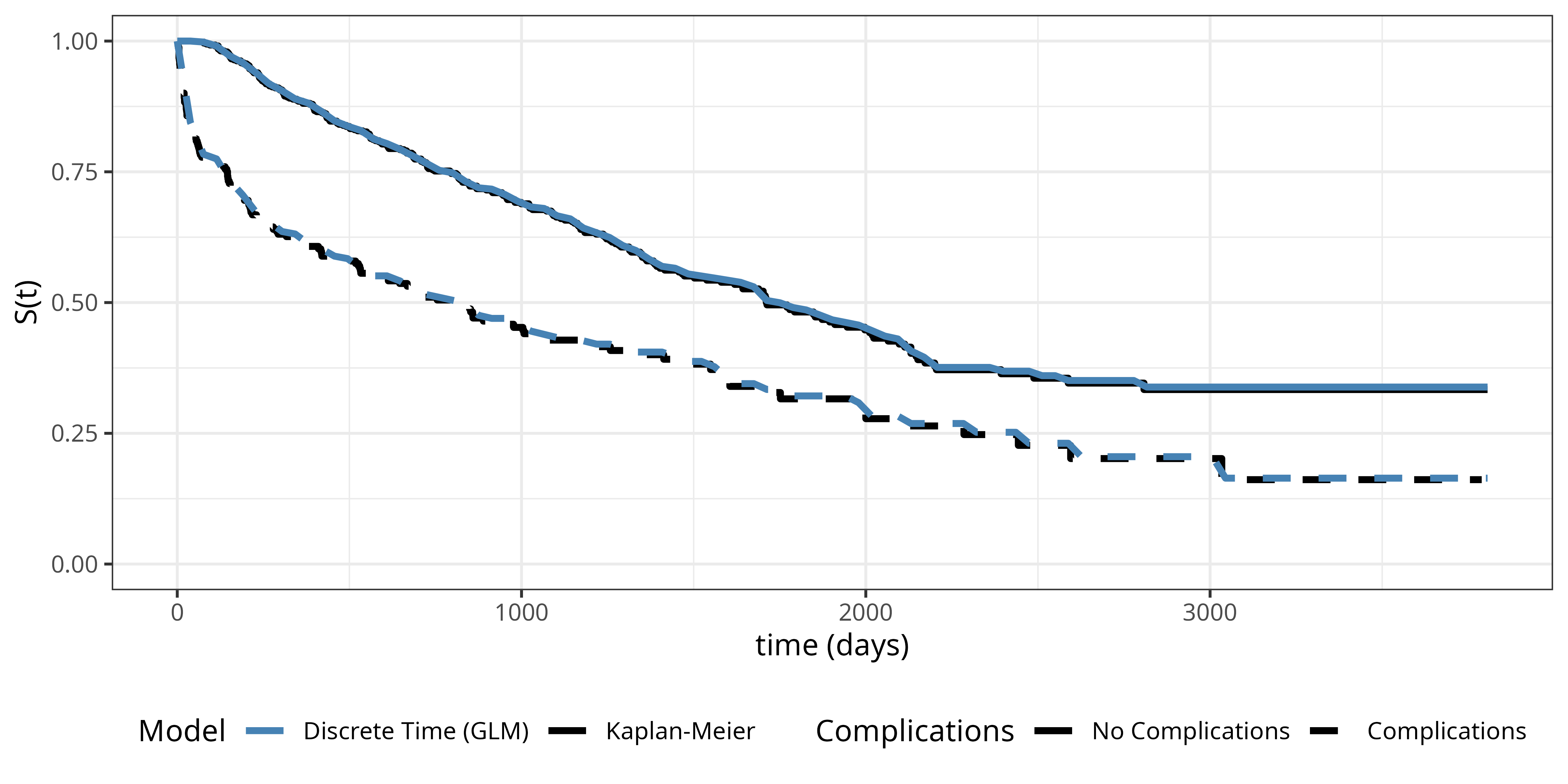
In order to estimate separate discrete baseline hazards for each group, we can introduce an interaction term between the interval and complications variables. \[\text{logit}(\pi_{ij}) = \beta_{0j} + \beta_{1j}x_{i1} \tag{18.12}\] where \(\beta_{0j}\) are the interval-specific intercepts for the reference group (no complications), \(\beta_{1j}\) are the deviations from the reference group for the complications group (technically this is fit as an interaction model using reference coded categorical features for interval and complications). This specification allows the shape of the hazard and therefore the survival probability curve to be different for the two groups.
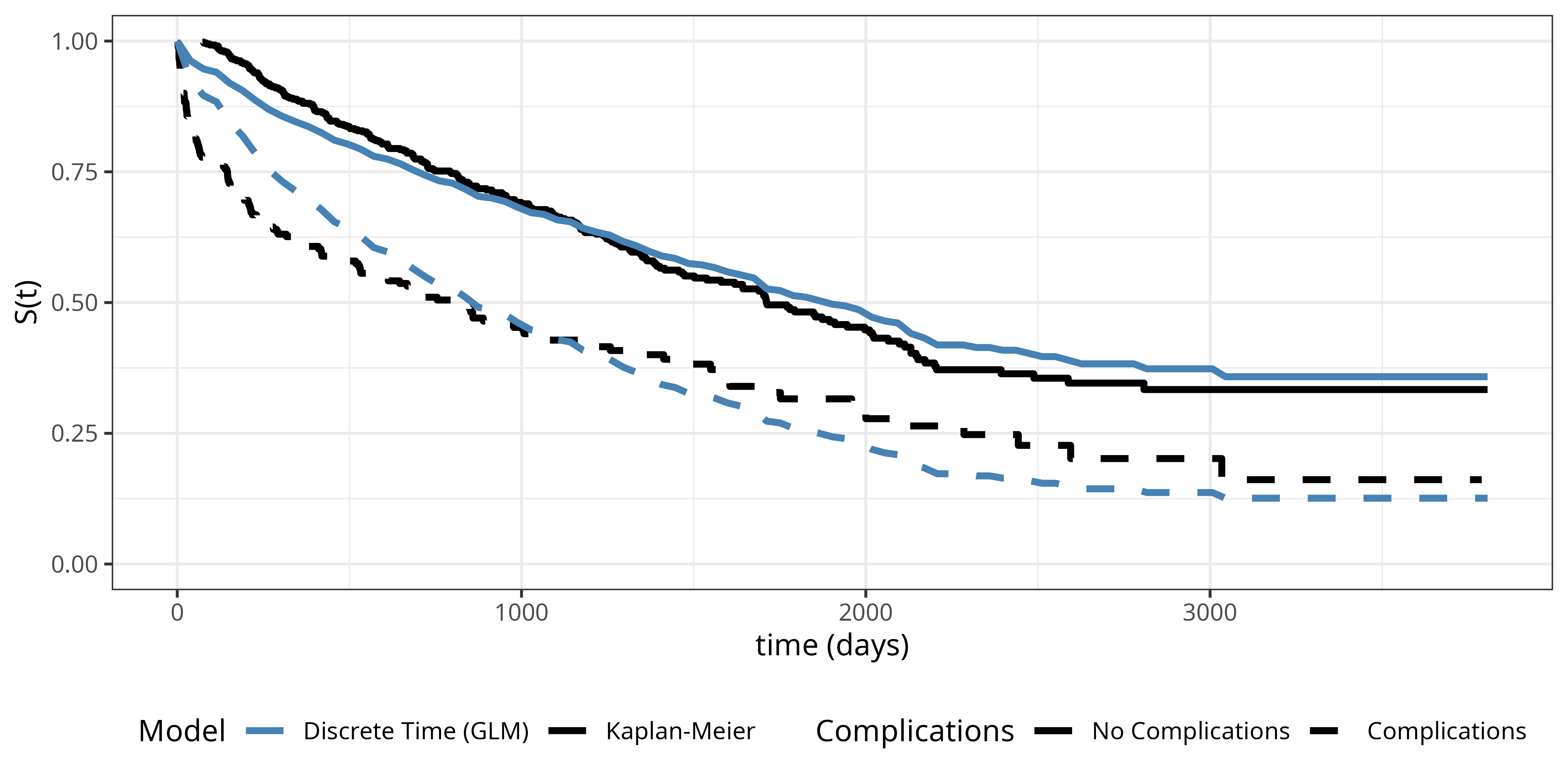
Figure Figure 18.4 shows the estimated survival probabilities from the interaction model (dashed lines) together with the Kaplan-Meier estimates (solid lines) for comparison. The interaction model provides a much better fit to the data compared to the proportional odds model, as it allows for separate baseline hazards for each complications group. The difference to the Kaplan-Meier estimates is barely detectable.
While this is a simple example with only one feature, it shows that the discrete time reduction approach can be used to estimate the distribution of event times well when the number of intervals is large enough, despite the fact that we ignore the information about the exact event time. Importantly, the estimated survival probabilities are discrete, representing survival probabilities at the interval endpoints. However, a simple solution to generate continuous survival function predictions is to linearly interpolate between the interval endpoints.
The example also raises the question about the choice of the number of intervals \(J\) and the placement of interval boundaries \(\mathcal{A}\). These questions will be discussed in more detail in Section 18.5, which is relevant for both, the discrete time reduction approach and the piecewise constant hazards approach discussed in Section 18.4.
18.3 Survival Stacking
Survival stacking (Craig et al. (2025)) casts survival tasks to classification tasks similarly to the discrete time method described in Section Section 18.2. However, there is a small but important difference in the creation of event indicators \(\delta_{ij}\). Rather than constructing intervals based on partitioning of the follow-up along boundary points \(\mathcal{A}\), survival stacking uses the unique, observed, ordered event times \(t_{(1)}, < \ldots < t_{(m)}\) (3.9) and defines \[\delta_{ij} = \begin{cases} 1, & t_i = t_{(j)} \text{ and } \delta_i = 1 \\ 0, & \text{ else } \end{cases},\quad j \in \{1,\ldots,m: i \in R_{t_{(j)}}\} \tag{18.13}\] where \(R_{t_{(j)}}\) is the risk set (3.10) at time \(t_{(j)}\).
Definition 18.13 implies that the event indicators \(\delta_{ij}\) are only defined for timepoints \(t_{(j)}\) at which subject \(i\) is still at risk for the event. Therefore, this method can be easily applied to left-truncated data by using the more general definition of the risk set (3.18).
For illustration, consider once again, the example from Figure Figure 18.2. The adapted data-transformation for survival stacking is shown in Figure Figure 18.5 (droping columns that are not meaningful here). At the first event time \(t_{(1)} = 0.5\), all subjects are sitll at risk for the event. At time \(t_{(2)} = 2.7\), however, only subject \(3\) is still at risk for the event.
Note that in contrast to Figure 18.2, here subject \(1\) has only one row and subject \(3\) has two rather than three rows. This could suggest that the data transformation for survival stacking creates smaller data sets, however, we need to create a data set for each observed event time \(t_{(j)}, j=1,\ldots,m\), whereas for the discret time approach in Section 18.2 one can freely choose the number and placement of interval boundaries \(\mathcal{A}\), such that \(|\mathcal{A}| < m\) in most cases.
Data transformation 18.13 yields data \[\mathcal{D}_{\mathcal{A}} = \{(\delta_{ij}, t_{j}, \mathbf{x}_{ij})\}_{i=1,\ldots,n;\ j=1,\ldots,m:\ i \in R_{t_{(j)}}}, \tag{18.14}\] where the \(\delta_{ij}\) can be used as targets for binary classification and as before, any algorithm that returns class probabilities can be used for estimation.
18.4 Piecewise Constant Hazards
The general idea of the piecewise constant hazards approach is conceptually simple:
- Partition the follow-up into many intervals
- Estimate a constant hazard rate for each interval
Intuitively, any underlying continuous hazard function of the data generating process can be approximated arbitrarily well given enough intervals (and events). This model class is known as the piecewise exponential model (PEM) because assuming event times to be exponentially distributed, implies constant hazards within each interval.
Consider the partitioning of the follow-up as defined in 18.1 and assume that within each interval \(I_j = (a_{j-1}, a_j]\), the hazard function is constant, that is \[h(\tau) = h_j,\ \forall\ \tau \in I_j \tag{18.15}\]
First we derive the likelihood contribution of subject \(i\) under assumption 18.15, starting with the general likelihood for right-censored data (3.12): \[\begin{aligned} \mathcal{L}_{i} & = h(t_i)^{\delta_{i}}S(t_i)\\ & = h(t_i)^{\delta_{i}}\exp\left(-\int_{0}^{t_i} h(u) \ \mathrm{d}u\right)\\ & = h_{J_i}^{\delta_{i}}\exp\left(-\left[\sum_{j=1}^{J_i-1} (a_j - a_{j-1})h_j + (t_i - a_{J_i-1})h_{J_i}\right]\right)\\ & = h_{J_i}^{\delta_{i}}\exp\left(-\sum_{j=1}^{J_i} h_j t_{ij}\right) = h_{J_i}^{\delta_{i}}\prod_{i=1}^{J_i}\exp\left(- h_j t_{ij}\right)\\ & = \prod_{j=1}^{J_i} h_j^{\delta_{ij}} \exp(-h_j t_{ij}), \end{aligned} \tag{18.16}\] where the first equality follows from 3.4, the third and fourth equalities follow from assumption 18.15 and definition 18.3, and the last equality follows from 18.2 such that \(h_{J_i}^{\delta_i} = \prod_{j=1}^{J_i} h_j^{\delta_{ij}}\) (when \(\delta_i = 0\), all \(\delta_{ij} = 0\), when \(\delta_{i} = 1\), only \(\delta_{iJ_i} = 1\)).
Now assume that the interval-specific event indicators \(\delta_{ij}\) are realizations of random variables \(\Delta_{ij} \stackrel{iid}\sim \text{Poisson}(\mu_{ij} : = h_j t_{ij})\) and recall that \(Z\sim \text{Poisson}(\mu)\) implies \(P(Z = z) = \frac{\mu^z \exp(-\mu)}{z!}\). Thus, the likelihood contribution of subject \(i\) can be written as \[\begin{aligned} \mathcal{L}_{\text{Poisson},i} & = \prod_{j=1}^{J_i} P(\Delta_{ij} = \delta_{ij}) = \prod_{j=1}^{J_i} \frac{(h_j t_{ij})^{\delta_{ij}} \exp(-h_j t_{ij})}{\delta_{ij}!}\\ & = \prod_{j=1}^{J_i} h_j^{\delta_{ij}} t_{ij}^{\delta_{ij}}\exp(-h_j t_{ij}), \end{aligned} \tag{18.17}\] where the last equality follows from \(\delta_{ij} \in \{0,1\}\) and \(0!=1!=1\).
Note that \(\mathcal{L}_{i,\text{Poisson}} \propto \mathcal{L}_i\) from equation 18.16, since \(t_{ij}\) is a constant and does not depend on the parameters of interest (here \(h_j\)). This implies that we can estimate a model with piecewise constant hazards by optimizing the Poisson likelihood 18.17. The \(t_{ij}\) term enters as an offset term \(\log(t_{ij})\) in the Poisson regression model.
More generally, in the presence of features \(\mathbf{x}_i\), assume \(\delta_{ij}|\mathbf{x}_i \stackrel{iid}{\sim} \text{Poisson}(\mu_{ij})\), where \(\mu_{ij} = h_{ij} t_{ij}\) is the expected number of events in interval \(j\) given features \(\mathbf{x}_i\) and \(h_{ij} = g(t_j, \mathbf{x}_i)\) is the hazard rate in interval \(j\) given features \(\mathbf{x}_i\). This can be estimated by fitting a Poisson regression model with log-link to the transformed data set \[\mathcal{D}_{\mathcal{A}} = \{(\delta_{ij}, t_{ij}, t_j, \mathbf{x}_{ij})\}_{i=1,\ldots,n; j=1,\ldots,J_i}, \tag{18.18}\] where the model specification is \[\log(\mathbb{E}[\Delta_{ij}]) = \log(h_{ij}) + \log(t_{ij}), \tag{18.19}\] where \(\log(h_{ij}) = g(\mathbf{x}_i, t_j)\) is the interval and feature specific hazard rate, \(g\) is a function learned by the model of choice and \(\log(t_{ij})\) is included as an offset term in the Poisson likelihood/Loss function.
Importantly, in contrast to the discrete time reductions in Section Section 18.2, the piecewise exponential model likelihood has no information loss regarding the exact time-to-event by including the \(t_{ij}\) terms (18.3) and estimates continuous time hazards rather than discrete time hazards.
18.4.1 Example: Poisson Regression
To illustrate the piecewise constant hazards approach, we once again consider the tumor data set. We partition the follow-up time into \(J = 100\) equidistant intervals. We then fit a Poisson regression model with interaction between interval and complications to allow for separate baseline hazards for each complications group:
\[\log(\mu_{ij}) = \log(\mathbb{E}[\Delta_{ij}]) = \underbrace{\beta_{0j} + \beta_{1j}x_{i1}}_{\log(h_{ij})} + \log(t_{ij}), \tag{18.20}\] where \(x_{i1} = \mathbb{I}(\text{complications}_i = \text{"yes"})\), \(\beta_{0j}\) are the interval-specific intercepts for the reference group (no complications), \(\beta_{1j}\) are the deviations from the reference group for the complications group (as in 18.12, this is estimated as an interaction model using reference coded categorical features for interval and complications), and \(\log(t_{ij})\) enters as offset term.
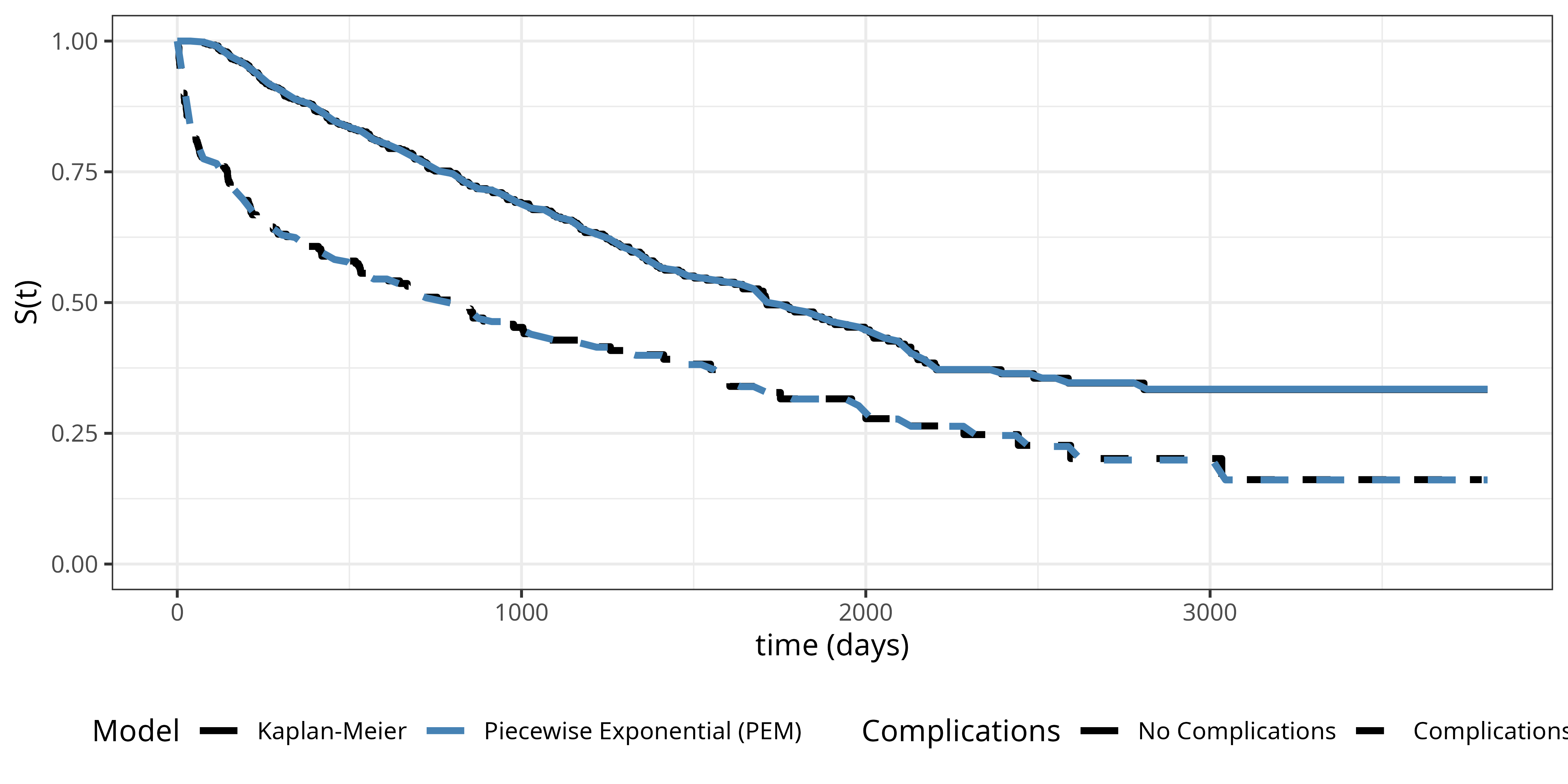
Figure Figure 18.6 shows the estimated survival probabilities from the piecewise exponential model (dashed lines) together with the Kaplan-Meier estimates (solid lines) for comparison. The piecewise exponential model provides an excellent fit to the data, closely approximating the Kaplan-Meier estimates. This demonstrates that the piecewise constant hazards approach can effectively estimate the survival distribution when using a sufficient number of intervals.