1 Introduction
Building on the motivation in the preface, this chapter introduces the concepts and terminology needed to specify a machine learning survival analysis problem:
- What distinguishes time-to-event data from data found in regression and classification;
- The prediction tasks unique to the survival setting; and
- The most common forms of censoring and truncation that appear in practice.
1.1 Survival analysis
This book uses the term survival analysis, which highlights the field’s roots in medical statistics, in particular the analysis of survival times (the time until death). However, as discussed in the preface, this is not the only application of the field and other terms may also be found; for example, reliability, duration, and failure-time analysis.
In Chapter 3, ‘survival analysis’ is refined to specifically refer to the case when the event of interest can occur exactly once, for example, predicting when a patient may die after diagnosis of Stage IV non-small cell lung cancer. In Chapter 4, ‘event history analysis’ is defined, which is a generalization of the single-event setting to the case when one or more events can occur one or more times, for example, predicting when a patient will have relapses of multiple sclerosis. To align with common practice, the term ‘survival analysis’ is used throughout the book and context will make clear when the more general event history methods apply.
One of the key aims in this book is to highlight the ubiquitous nature of survival analysis and to encourage more machine learning practitioners to use it when appropriate. Machine learning practitioners are likely familiar with classification and regression, but may not be familiar with survival analysis. The examples below demonstrate when survival analysis might be appropriate.
Survival probabilities
Returning to the example in the preface, say an elderly man receives the treatment investigated in the randomized trial for advanced non-small cell lung cancer (NSCLC). The oncologist might tell him (in softer words) “based on the results of this trial, the three-year survival probability of NSCLC in 75-year-old males on this treatment is 67.5%”. This initially appears as a probabilistic classification problem: given a set of patient characteristics (here age and sex), predict whether a patient survives to three years (a binary outcome). In other words, among patients with similar characteristics, approximately 67.5% survived to three years. However, the data needed to estimate such probabilities is obtained from a dataset with incomplete information. For many patients, the event time is only partially observed. For example, a patient may withdraw from the study for unrelated reasons, become lost to follow-up, or remain alive when the study ends at a fixed cutoff date. These situations are examples of right-censoring events. Treating an observation that was censored as a negative label (that is, “the event did not occur”) in a classification model would introduce bias. Survival analysis models allow valid estimation of the three-year survival probability by taking into account the information from all observations, including the censored ones.
Risk score calculation
Another common survival problem is to rank observations rather than predicting an absolute probability. Consider the allocation of donor hearts to eligible candidates on a transplant waiting list, which requires estimating which candidate is most likely to die soonest without a transplant. Candidates could be ranked in a list of lowest to highest risk of death, or assigned to risk groups: for example, patients at low or high risk of dying within one year. A naive approach would be to train a classification model on historical waiting-list data, labeling each patient as “died within one year” or “survived to one year”. However, waiting-lists contain many censored records and competing events: some patients will receive a transplant before the one-year mark (hence their natural waiting-list outcome is no longer observable after transplant) and others will be lost to follow-up or remain on the list at the end of the study. A classifier restricted to patients with a fully observed one-year outcome may discard the cases that most inform the ranking and thus yield biased predictions. A survival model uses the partial information in censored records to produce a risk ranking that reflects the relative ordering of event times (under appropriate assumptions about the censoring process).
Estimating duration
For a non-medical example, return to the study in the preface that considered how long unemployed workers take to find a full-time job (assuming the outcome is first exit from current unemployment period). Say data is collected over one calendar year. At the end of that period, many workers will still be unemployed, while others may move to a different country, take on a part-time job, be permanently removed from the labor force, or drop out of the study for other reasons. A regression model trained only on uncensored observations could be heavily biased because the longest unemployment spells, those ongoing at the study end, would be absent from the training data.
This unemployment setting has further structure that standard regression cannot accommodate. Workers may exhibit multiple unemployment spells (recurrent events) and the ways in which they exit unemployment may be mutually exclusive: someone cannot both find full-time work and be permanently removed from the workforce. Treating only one exit type as the event of interest and lumping the others in with censoring would mis-specify the problem; a more appropriate analysis would use competing risks or multi-state models (Chapter 4).
These examples also demonstrate the nuance of a survival analysis prediction (Chapter 5), which may involve predicting the probability of an event at a certain time (survival probabilities), ranking observations within a sample (risk scores), or estimating the time until an event takes place (duration).
1.2 Machine learning survival analysis
Machine learning is an interdisciplinary field primarily concerned with building models that learn structure from data, for example to predict outputs from inputs or to identify patterns within observed data (Hastie et al. 2001). Defining if a model should be called ‘machine learning’ is surprisingly difficult; there is no clear boundary separating straightforward statistical models from what is now often termed machine learning. This book defines machine learning in a pragmatic sense to denote models whose parameters or structure are learned from data by optimizing an explicit objective function and whose success is judged by empirical performance on unseen data. This definition tightly couples the concept of machine learning with the need for robust evaluation (Part II) and allows for a broad range of models (Part III) to be considered machine learning, including those that would commonly be considered statistical models.
This book focuses on the supervised learning setting, where the goal is to predict outcomes from labeled training data. Development of machine learning survival analysis models has converged on three primary tasks of interest (formally defined in Chapter 5), or survival problems, which are defined by the type of prediction the model makes. Generally, a survival problem arises when a model is trained on censored data to predict one of:
- A survival distribution: The probability distribution over event times.
- A relative risk: The risk of an event taking place compared to other observations in the same sample.
- A survival time: A predicted event time.
Each prediction type serves a different purpose and a practitioner may be required to develop multiple models for optimal estimation of each prediction type. As an example, an engineer is unlikely to care about the exact time at which a plane engine fails, but they might greatly value knowing when the probability of failure increases above 5%, which is a survival distribution prediction. Returning to the transplant example, clearly choices cannot be easily made on a full survival distribution for every candidate on the waiting list, but an allocation can be made if it is clear one candidate is at substantially greater risk of death in the near term than another, a relative risk prediction. As will be seen in Chapter 5, these tasks are mathematically related and, subject to certain assumptions, may be transformed into one another.
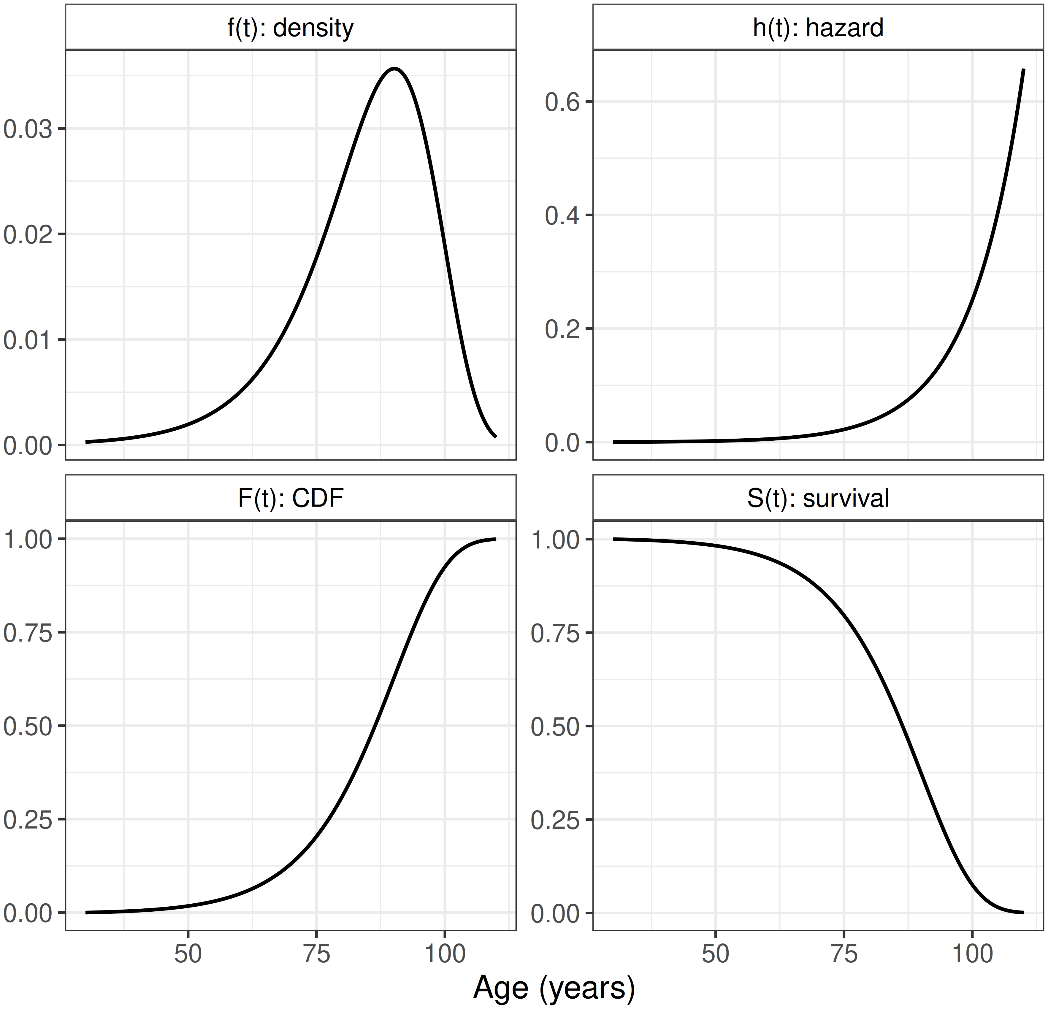
When it comes to making distribution predictions, survival analysis stands out again. Common distribution-defining functions used to characterize probability distributions, are the probability density function (for continuous distributions) and the cumulative distribution function (CDF). In survival settings, interpreting the density function can be counter-intuitive because it is an unconditional density over event times measured from a common time origin, such as diagnosis or treatment initiation. In other words, it describes how event times are distributed when following individuals forward from a shared starting point. The CDF is the probability that the event has ‘already’ taken place at a given time, which is opposite to the usual survival prediction: whether the event ‘will’ take place. Therefore, survival analysis focuses instead on predicting the survival function, which is simply one minus the CDF, and the hazard function. Unlike the density function, which describes the unconditional distribution of event times from baseline, the hazard function describes the instantaneous risk of the event at a given time conditional on having survived up to that time.
These functions are formally defined in Chapter 3 and are visualized in Figure 1.1 using a Gompertz distribution, often used to model adult lifespans, fit to Swedish mortality data (Broström 2024). The survival function (bottom right) decreases from one to zero and gives the probability of surviving to a given age (equivalently, that death has not occurred by that age); the cumulative distribution function (bottom left) is its mirror image. The density (top left) peaks around age 88, which is the age at which unconditional deaths are most common. The hazard (top right) is a conditional rate and is not bounded above by one; on this fit it doubles roughly every seven years and is still climbing steeply at the oldest ages. Because the time axis is age in years, the hazard has units of per year. For example, the fitted hazard is approximately \(0.08\)/yr at age 88 (\(\approx 8\%\) chance of dying within the next year given survival to 88). To help exemplify the difference between the density and hazard, consider the risk of death at age 100. Given that someone is alive at 100, their instantaneous risk of death (hazard) is approximately \(3\) times higher than at age 88. In contrast, the event-time density around age 100 is half the density at age 88, as far fewer individuals survive to age 100 overall.
1.3 Censoring and truncation
As already discussed, censoring is a defining feature of survival analysis. In addition to censoring, survival data can include truncation, which means portions of follow-up time are excluded. The precise definitions of the different types of censoring and truncation are provided in Chapter 3. Brief, non-technical summaries are given below.
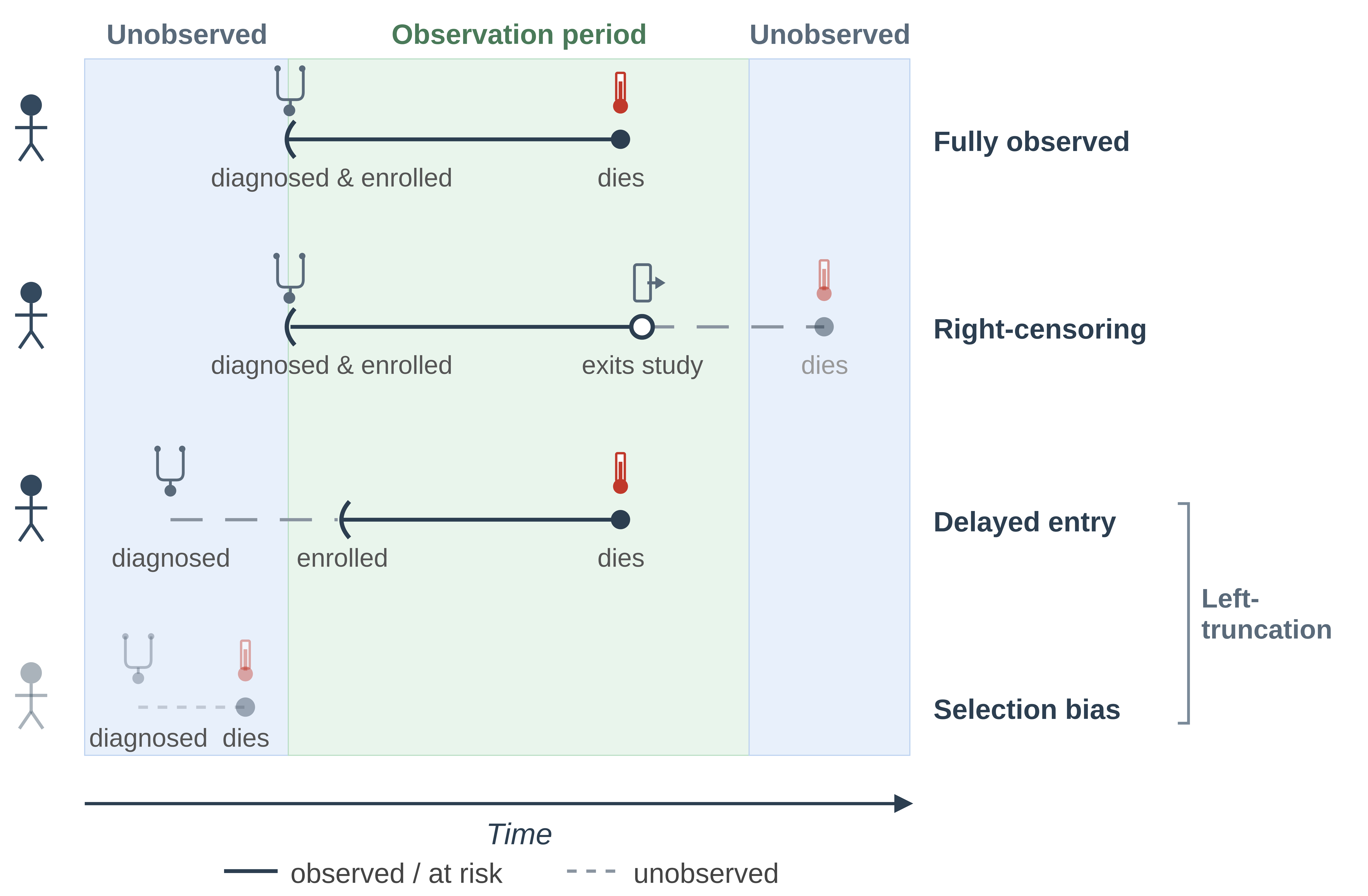
The most common form of censoring is right-censoring (Figure 1.2, second row), which occurs when the true survival time is greater than (‘to the right of,’ if you imagine a number line) the observed censoring time. The examples in Section 1.1 all exhibit forms of right-censoring. Left-censoring is recorded when the event of interest is less than (‘to the left of’) the observed censoring time. Chapter 3 provides an example of someone telling an interviewer that they started using a phone (the event of interest) before the interview, but they do not remember when. If the time-to-event outcome is “age at first phone use” then a \(23\)-year-old who is using a phone but cannot remember when they started is left-censored at \(23\). Often, the censoring event is assumed to be independent of the event of interest (for example, random dropout). However, when the occurrence of another event precludes observation of the primary event, it is known as a competing risk (Chapter 4). For example, if an unemployed worker is still looking for a job when the study window closes, the reason for censoring is independent of the outcome. In contrast, finding a part-time job is a competing event as it precludes the primary event (finding full-time employment) and may depend on the same factors (skills, availability, local labor market).
Left-truncation is the more common form of truncation and involves data before the truncation time being excluded. Left-censoring occurs because the event of interest has already occurred, but the exact time is unknown. Left-truncation happens when subjects experience the event before meeting the inclusion criteria and thus never enter the study at all. Truncation affects whether an individual is included in the observed sample, whereas censoring affects how much of an included individual’s outcome time is observed.
As a concrete example, consider a study on time until death in patients diagnosed with tuberculosis (TB). Assume enrollment is open to anyone with a TB diagnosis, including those diagnosed before the study opened. Left-truncation arises if patients die between their diagnosis and the study start. These patients are never observed and are absent from the data, inducing a form of selection bias: the highest-risk cases (those dying earliest) are systematically missing (Figure 1.2, fourth row). Those who do survive to the study start will enter with a known gap between diagnosis and enrollment (Figure 1.2, third row). Bias occurs when delayed entry and the implicit selection bias are not explicitly accounted for (discussed in full in Chapter 3).
Another bias that often occurs when time-dependent dynamics of survival data collection are not explicitly accounted for is immortal time bias. This occurs when group membership (treatment) is determined only after a period of guaranteed survival but is treated as if present from baseline. Immortal time bias is also discussed further in Chapter 3.
The first part of this book will formally introduce and develop these concepts further.