14  Gradient Boosting Machines

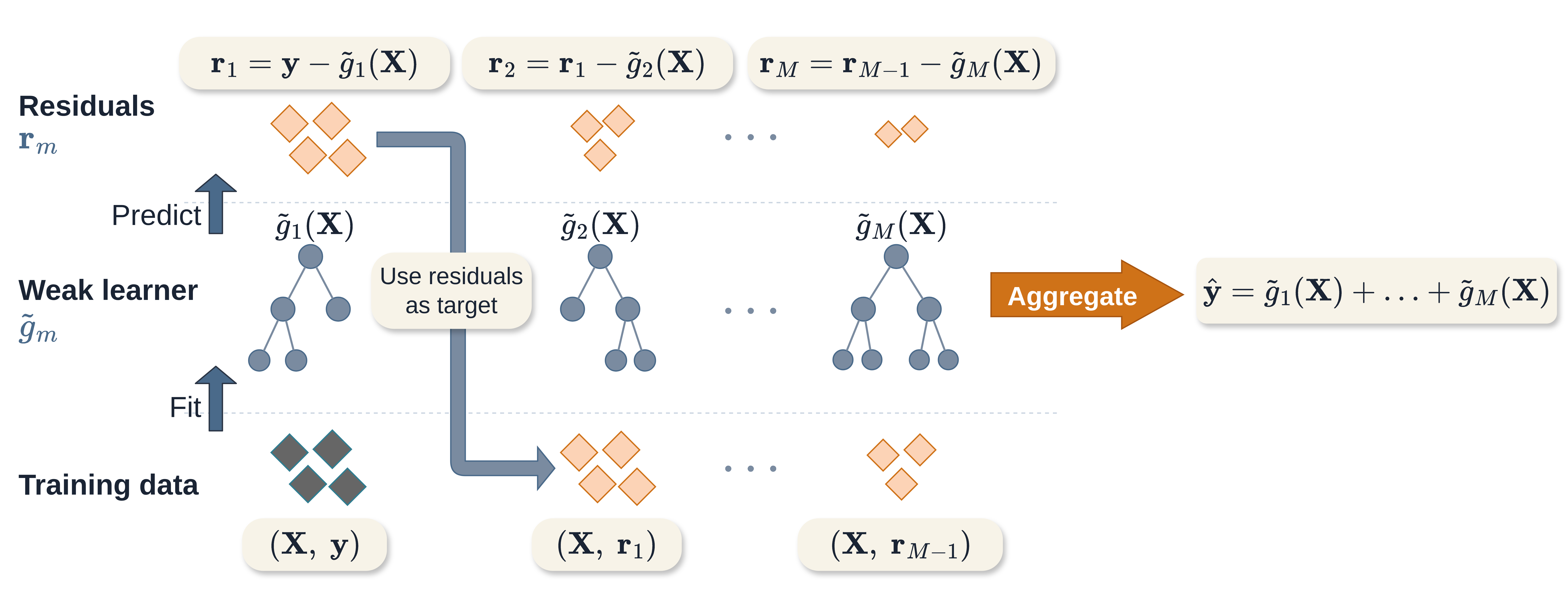
Similarly to random forests, boosting is an ensemble method that creates a powerful model from a combination of weak learners that make poor predictions individually. However, the two methods differ in how individual learners are selected and combined: in random forests, each decision tree is grown independently and predictions are averaged. In boosting, weak learners are fit sequentially with errors from one learner used to train the next, and predictions are made by a weighted linear combination of all learners (Figure 14.1).

14.1 GBMs for regression

Gradient boosting machines (GBMs) are among the most widely used families of boosting algorithms. The general idea, inspired by gradient descent (Section 2.6.1), is to choose a differentiable loss function and iteratively improve predictions by fitting weak learners to the remaining errors from the current model. These errors correspond to the negative gradients, or pseudo-residuals. Figure 14.1 illustrates this process in a least-squares regression setting, where the negative gradient corresponds to the ordinary residual, which is the observed outcome minus the current prediction. This procedure can be understood as follows:

1. An initial, simple model is fit to the data to obtain the first set of predictions.
2. The errors of this model are computed by comparing predictions to the observed outcomes.
3. A weak learner is fit to these errors, focusing on patterns that the previous model failed to capture.
4. The new learner is added to the existing model, improving the overall prediction.
5. This is repeated with each learner correcting the errors of the current model.

Predictions are therefore built up gradually as a sum of many weak learners, each making a small contribution to the final model.

Figure 14.1: Least squares gradient boosting, where each weak learner (here, a decision tree) is fit to the residuals (negative gradient of squared error loss).

Practically, a number of important hyperparameters are used to control and optimize the algorithm while reducing overfitting. These are:

Number of iterations, \(M\): The number of iterations is often claimed to be the most important hyperparameter in GBMs and it has been demonstrated that a value too small will result in underfitting, while a value too large will result in overfitting (Buhlmann 2006; Hastie et al. 2001; Schmid and Hothorn 2008a). This underlines the general idea of boosting weak learners to slowly construct a single powerful model.

Step size, \(\alpha\): The step size parameter is a shrinkage parameter that controls the contribution of the weak learner at each iteration. Several studies have demonstrated that GBMs perform better when shrinkage is applied and a value of \(\alpha \leq 0.1\) is often suggested (Buhlmann and Hothorn 2007; Friedman 2001; Hastie et al. 2001; Lee et al. 2021; Schmid and Hothorn 2008a). The optimal values of \(\alpha\) and \(M\) depend on each other, such that smaller values of \(\alpha\) require larger values of \(M\), and vice versa. This is intuitive as smaller \(\alpha\) results in slower learning and therefore more iterations are required to fit the model. A practical procedure is to set \(\alpha\) to a small value (such as \(0.1\)) and \(M\) to a very large value (such as \(10,\!000\)), then use early stopping (Section 2.6.2) to halt the algorithm once performance on a validation set stops improving. This avoids the need for computationally expensive tuning to find the optimal combination of \(\alpha\) and \(M\).

Subsampling proportion, \(\phi\): Sampling a fraction, \(\phi\), of the training data at each iteration can improve performance and reduce runtime (Hastie et al. 2001), with \(\phi = 0.5\) often used although ideally it should be tuned. Motivated by the success of bagging in random forests, stochastic gradient boosting (Friedman 1999) randomly samples the data in each iteration. Subsampling appears to perform best when combined with shrinkage (Hastie et al. 2001).

In addition to these parameters, the hyperparameters of the underlying weak learner are also commonly tuned. When using decision trees, it is usual to restrict the number of terminal nodes in the tree to be between \(4\) and \(8\), which corresponds to two or three splits in the tree. With these hyperparameters and some differentiable loss \(L\), the general gradient boosting machine algorithm is given in Algorithm 2.

NoteAlgorithm 2 (Gradient boosting)

1. \(\hat{g}_0 \gets \text{ Initial guess}\)
2. for \(m = 1,\ldots,M\):
3.      \(\{(\mathbf{x}_i', y_i')\}^{n'}_1 \gets\) Random sample of size \(n' = \lfloor \phi n \rfloor\) from \(\{(\mathbf{x}_i, y_i)\}_1^n\)
4.      \(\displaystyle r_{im} \gets -\frac{\partial L(y'_i, \hat{g}_{m-1}(\mathbf{x}'_i))}{\partial \hat{g}_{m-1}(\mathbf{x}'_i)}, \forall i \in \{1,\ldots,n'\}\)
5.      \(\tilde{g}_m \gets\) Fit the weak learner to \((\mathbf{X}', \mathbf{r}_m)\)
6.      \(\hat{g}_m \gets \hat{g}_{m-1} + \alpha \tilde{g}_m\)
7. end for
8. return \(\hat{g}_0, \{\tilde{g}_m\}^M_1\)

Note:

1. \(\tilde{g}_m\) is the weak learner in iteration \(m\) trained on pseudo-residuals computed from the cumulative model from the previous iteration, \(\hat{g}_{m-1}\). The returned object can be written as the final cumulative model, \(\hat{g}_M\), although in practice the model is computationally stored as the set of trained learners.
2. The initial guess (or offset), \(\hat{g}_0\), is often the best constant prediction under the chosen loss, \(\hat{g}_0 = \mathop{\mathrm{arg\,min}}_c \sum_{i=1}^n L(y_i, c)\). For regression, using the mean squared error loss reduces to the mean of the training data, \(\hat{g}_0 = \bar{y}\).
3. Line 4 is the calculation of the negative gradient (Section 2.6.1), which is equivalent to calculating the residuals in a regression problem with the mean squared error loss.
4. Lines 5–6 differ between implementations, with some fitting multiple weak learners and selecting the one that minimizes the objective function. When candidate learners are fit separately to individual features, this is known as componentwise boosting; see Further Reading for references. The version above is conceptually simplest and straightforward to implement, while still providing good model performance.

Once the model is trained, predictions are made for new data, \(\mathbf{x}_*\) with:

\[ \hat{g}_M(\mathbf{x}_*) = \hat{g}_0 + \alpha \sum^M_{m=1} \tilde{g}_m(\mathbf{x}_*). \]

GBMs provide a flexible, modular algorithm, primarily composed of a differentiable loss to minimize, \(L\), and the selection of weak learners. Perhaps the most common weak learners are decision trees, linear least squares (Friedman 2001) and smoothing splines (Bühlmann and Yu 2003). Trees allow the structure of the resulting prediction function to vary substantially; for example, using stumps (trees with only one split) results in an additive model with main effects only, whereas decision trees with an extra layer yield two-way interactions. This chapter focuses on tree-based learners, which are primarily used for survival analysis, due to the flexibility demonstrated in Chapter 12. See references at the end of the chapter for other weak learners.

14.2 GBMs for survival analysis

Unlike other model classes, survival analysis was considered in early GBM papers (Ridgeway 1999), although there appears to have been a decade-long gap before further advances were made. Subsequently, Hothorn et al. (2005), Schmid and Hothorn (2008b), Schmid and Hothorn (2008a), and Binder and Schumacher (2008) further developed GBM frameworks for survival analysis, which are discussed in this chapter.

In principle, boosting could be applied to models that directly predict a full survival distribution by optimizing a proper scoring rule (Chapter 8). However, standard boosting updates a single real-valued function at each iteration by fitting to the residual errors. When the target is a full survival distribution, scoring rules aggregate prediction errors across time, making it difficult to attribute errors to specific regions of the prediction and construct effective updates. This may partly explain why boosting methods in survival analysis are often applied to models that produce scalar risk scores.

This section begins with boosting approaches based on the core models introduced in Chapter 11, specifically proportional hazards (PH) and accelerated failure time (AFT) models (Section 14.2.1). In the case of the AFT models, the model parameters are estimated directly, which specifies a full survival distribution prediction. The discussion then extends to approaches that do not assume a specific model form, but instead directly optimize discriminatory ability by using a concordance index (Chapter 6) as the loss (Section 14.2.2).

14.2.1 Likelihood boosting

The negative log-likelihood of the semi-parametric PH and fully-parametric AFT models can be derived from the (partial) likelihoods presented in Section 11.2.2 and Section 11.3 respectively.

14.2.1.1 Cox proportional hazards boosting

To boost a Cox-type model, at each iteration, the weak learner in Algorithm 2 is taken to be a linear predictor,

\[ g_m(\mathbf{x}_i) = \eta_{m;i} = \mathbf{x}_i^\top\boldsymbol{\beta}_m, \tag{14.1}\]

where \(\eta_{m;i}\) is the updated linear predictor in iteration \(m\) and \(\eta_{0;i} = 0\).

Recall the Cox partial likelihood (11.7) given by (Cox 1972, 1975),

\[ \mathcal{L}_{PL}(\boldsymbol{\beta}) = \prod_{k=1}^{\tilde{n}} \left(\frac{\exp(\eta_{i_{(k)}})}{\sum_{j \in \mathcal{R}_{t_{(k)}}} \exp(\eta_j)}\right), \]

with corresponding negative log-likelihood (11.8):

\[ -\ell_{PL}(\boldsymbol{\beta}) = -\sum_{k=1}^{\tilde{n}} \left(\eta_{i_{(k)}} - \log \left(\sum_{j \in \mathcal{R}_{t_{(k)}}} \exp(\eta_j)\right)\right), \tag{14.2}\]

where \(t_{(k)}\) is the \(k\)th ordered event time for \(\tilde{n} < n\) event times, \(\mathcal{R}_{t_i}\) is the set of patients at risk at time \(t_i\) (assuming no ties).

The negative gradient of \(-\ell_{PL}(\boldsymbol{\beta})\) at iteration \(m\) is then given by substituting (14.1) for \(\eta_i\) into the negative log-likelihood (14.2) and differentiating (Ridgeway 1999):

\[ r_{im} := \delta_i - \sum^{\tilde{n}}_{k=1} \frac{\mathbb{I}(t_i \geq t_{(k)}) \exp(\hat{g}_{m-1}(\mathbf{x}_i))}{\sum_{j \in \mathcal{R}_{t_{(k)}}} \exp(\hat{g}_{m-1}(\mathbf{x}_j))}. \]

14.2.1.2 Accelerated failure time boosting

For non-PH data, boosting an AFT model can outperform boosted PH models (Schmid and Hothorn 2008b). Recall from Section 11.3 the log-linear AFT model (11.23) defined by:

\[ \log(t_i) = \mu + \eta_i + \sigma\epsilon_i, \]

where \(\sigma\) is a scale parameter, \(\epsilon_i\) is an error term, and \(\mu\) is an intercept. The model is now boosted by updating

\[ \hat{g}_m(\mathbf{x}_i) = \mu + \eta_i, \]

and then estimating \(\hat{\sigma}_m\) using the updated \(\hat{g}_m\); usually \(\sigma_0 = 1\) (Schmid and Hothorn 2008b). Rearranging (11.23) in terms of \(\epsilon_i\) and \(\hat{g}\) gives,

\[ \epsilon_i = \frac{\log(t_i) - \hat{g}_m(\mathbf{x}_i)}{\sigma}. \tag{14.3}\]

By assuming a distribution on \(\epsilon_i\), a distribution is assumed for the full parametric distribution of the survival time, giving the AFT log-likelihood (Klein and Moeschberger 2003),

\[ \begin{aligned} -l^{AFT}(g, \sigma) & = -\sum^n_{i=1} \Bigg[ \delta_i\Bigg(- \log{\sigma} + \log f_{\epsilon}\Big(\frac{\log(t_i) - g(\mathbf{x}_i)}{\sigma}\Big)\Bigg) \\ & + (1-\delta_i)\Bigg(\log S_{\epsilon}\Big(\frac{\log(t_i) - g(\mathbf{x}_i)}{\sigma}\Big)\Bigg) \Bigg] \end{aligned}, \tag{14.4}\]

where \(f_{\epsilon}, S_{\epsilon}\) are the density and survival functions of \(\epsilon\) respectively assuming a shared error distribution for all observations, and the expressions within \(f_{\epsilon}\) and \(S_{\epsilon}\) are a substitution of the error term (14.3). At iteration \(m\), (14.4) is evaluated at \((\hat{g}_{m-1}, \hat{\sigma}_{m-1})\) to compute the pseudo-residuals used to update \(\hat{g}_m\) following Algorithm 2,

\[ r_{im} = -\frac{\partial(-l^{AFT}(\hat{g}_{m-1}, \hat{\sigma}_{m-1}))}{\partial \hat{g}_{m-1}(\mathbf{x}_i)}. \]

The only change to the algorithm is a final step in each iteration where the scale parameter is re-estimated conditional on the updated \(\hat{g}_m\), by minimizing (14.4) with respect to \(\sigma\):

\[ \hat{\sigma}_m := \mathop{\mathrm{arg\,min}}_{\sigma > 0} \ -l^{AFT}(\hat{g}_m, \sigma), \]

which is the conditional maximum likelihood estimate of \(\sigma\) given the current boosted fit and is usually obtained by a one-dimensional numerical optimization over \(\sigma > 0\).

As well as boosting fully-parametric AFTs, one could consider boosting semi-parametric AFTs, for example, with the Gehan loss (Johnson and Long 2011) or using Buckley-James imputation (Wang and Wang 2010). However, known problems with semi-parametric AFT models and the Buckley-James procedure (Wei 1992), as well as a lack of off-the-shelf implementation, mean that these methods appear to be rarely used in practice.

The flexibility of boosting allows extensions to other censoring and truncation types to follow simply by replacing the likelihood functions above with the corresponding objective functions in Section 3.5.1.

14.2.1.3 Penalized boosting

‘CoxBoost’ (Binder and Schumacher 2008) is an alternative method to boost Cox models and has been demonstrated to perform well in experiments (Burk et al. 2026). The algorithm can be interpreted as a componentwise boosting procedure for Cox models, where at each iteration a single covariate is selected, alongside mandatory (or ‘forced’) covariates, and coefficients are updated using a penalized second-order optimization step (Binder and Schumacher 2008). In medical domains the inclusion of mandatory covariates may be essential, either for model interpretability, or due to prior expert knowledge. CoxBoost deviates from Algorithm 2 by instead using an offset-based approach for generalized linear models (Tutz and Binder 2007).

As this method is more technically involved than standard gradient boosting, consider the following motivational example (Table 14.1). Suppose treatment group is considered clinically essential and must always be included in the model, while age and a biomarker are optional covariates. In each boosting iteration, CoxBoost considers candidate updates componentwise by adding one optional covariate at a time to the mandatory covariate. In this example, the two candidate updates are therefore treatment group with age or treatment group with the biomarker. At each iteration, the candidate update with the lower loss (in bold) is selected and added to the coefficient vector. For example, in iteration \(1\), the update using age gives a lower loss than the update using the biomarker, so the coefficients for treatment group and age are updated. In iteration \(2\), the update using the biomarker gives a lower loss, so the coefficients for treatment group and the biomarker are updated instead. The optional covariate that is not selected in a given iteration is left unchanged. The running coefficient vector \(\hat{\boldsymbol{\beta}}_m\) plays the same role as the cumulative boosted predictor \(\hat{g}_m\) in Algorithm 2. The vector \(\hat{\boldsymbol{\gamma}}_{mk}\) is the candidate increment being considered in iteration \(m\) for candidate set \(k\). For the selected candidate \(k^*\), \(\hat{\boldsymbol{\gamma}}_{mk^*}\) is added to \(\hat{\boldsymbol{\beta}}_{m-1}\) to obtain \(\hat{\boldsymbol{\beta}}_m\), analogous to adding the new learner contribution \(\alpha \tilde{g}_m\) in standard gradient boosting.

Table 14.1: Three iterations of the CoxBoost algorithm with one mandatory covariate ‘trt’ and two optional covariates ‘age’ and ‘bio’. First column is iteration number, with one row per candidate optional covariate. Second column is the covariate under consideration with the resulting loss in third column (bold is the smaller loss and therefore the selected covariate). Columns four and five are the incremental updates in iteration \(m\) to the mandatory covariate and the selected optional covariate; in practice, increments are estimated for all candidate sets in each iteration, but only the increments for the selected candidate \(k^*\) are shown here for clarity. Columns six to eight are the accumulated coefficients for all covariates.

\(m\)	Candidate covariate	Loss after update	\(\hat{\gamma}_{mk^*,\text{trt}}\)	\(\hat{\gamma}_{mk^*,\text{opt}}\)	\(\hat{\beta}_{m,\text{trt}}\)	\(\hat{\beta}_{m,\text{age}}\)	\(\hat{\beta}_{m,\text{bio}}\)
0	–	–	–	–	0.00	0.00	0.00
1	Age	1.42	0.08	0.15	0.08	0.15	0.00
1	Biomarker	1.55	–	–	0.08	0.15	0.00
2	Age	1.31	–	–	0.08	0.15	0.00
2	Biomarker	1.20	0.03	0.20	0.11	0.15	0.20
3	Age	1.11	-0.02	0.06	0.09	0.21	0.20
3	Biomarker	1.18	–	–	0.09	0.21	0.20

After the final iteration in Table 14.1, the fitted model for observation \(i\) is therefore

\[ \hat{h}(\tau \mid \mathbf{x}_i) = \hat{h}_0(\tau)\exp(0.09x_{i,\mathrm{trt}} + 0.21x_{i,\mathrm{age}} + 0.20x_{i,\mathrm{bio}}), \]

where the coefficients are the final accumulated values in \(\hat{\boldsymbol{\beta}}_3\).

To formally introduce the model, let \(\mathcal{I}= \{1,\ldots,p\}\) be the indices of the covariates, let \(\mathcal{I}_{\text{mand}}\) be the indices of the mandatory covariates that must be included in all iterations, and let \(\mathcal{I}_{\text{opt}} = \mathcal{I}\setminus \mathcal{I}_{\text{mand}}\) be the indices of the optional covariates that may be included in any iteration. In each iteration, the algorithm considers models that include all mandatory covariates together with a single optional covariate, selecting the covariate that yields the greatest improvement in the penalized likelihood:

\[ \mathcal{I}_{mk} = \mathcal{I}_{\text{mand}} \cup \{k\}, \quad k \in \mathcal{I}_{\text{opt}}. \]

In addition, a penalty matrix \(\mathbf{P} \in \mathbb{R}^{p \times p}\) is considered such that \(P_{ii} > 0\) implies that covariate \(i\) is penalized and \(P_{ii} = 0\) means no penalization. In practice, this is usually a diagonal matrix (Binder and Schumacher 2008) and by setting \(P_{ii} = 0, i \in \mathcal{I}_{\text{mand}}\) and \(P_{ii} > 0, i \not\in \mathcal{I}_{\text{mand}}\), only optional (non-mandatory) covariates are penalized. The penalty matrix can vary with each iteration, which allows for a highly flexible approach. In practice, a simpler approach is to use the same penalty matrix in each iteration and to apply the same penalty factor to all penalized covariates (Binder 2013).

At the \(m\)-th iteration and the \(k\)-th set of indices to consider, the loss to optimize is the penalized partial log-likelihood given by,

\[ \begin{aligned} &l_{pen}(\boldsymbol{\gamma}_{mk}) = \\ &\sum_{\tau=1}^{\tilde{n}} \left[\eta_{i_{(\tau)},m-1} + \mathbf{x}_{i_{(\tau)},\mathcal{I}_{mk}}^\top\boldsymbol{\gamma}_{mk} - \log\left(\sum_{j \in \mathcal{R}_{t_{(\tau)}}} \exp\left(\eta_{j,m-1} + \mathbf{x}_{j,\mathcal{I}_{mk}}^\top\boldsymbol{\gamma}_{mk}\right)\right)\right] - \lambda\boldsymbol{\gamma}^\top_{mk}\mathbf{P}\boldsymbol{\gamma}_{mk}. \end{aligned} \tag{14.5}\]

where \(\eta_{i,m} = \mathbf{x}_i^\top\boldsymbol{\beta}_m\), \(\boldsymbol{\gamma}_{mk}\) are the coefficient updates corresponding to the candidate covariate set \(\mathcal{I}_{mk}\), \(\mathbf{P}\) is the penalty matrix (assuming the same in every iteration), \(\lambda\) is a penalty hyperparameter, and \(t_{(\tau)}\) is the \(\tau\)th ordered event time for \(\tilde{n} < n\) unique event times (assuming no ties).

In each iteration, all potential candidate sets are considered and the optimal set is the one that results in the largest improvement in the penalized partial log-likelihood. Note that CoxBoost uses Fisher scoring iterations to update the coefficient estimates, using both first and second derivatives, whereas standard GBMs only use first derivatives.

The optimal set is then found as,

\[ k^* := \mathop{\mathrm{arg\,max}}_k \ l_{pen}(\hat{\boldsymbol{\gamma}}_{mk}), \]

and the estimated coefficients are updated by,

\[ \hat{\beta}_{m, j} = \begin{cases} \hat{\beta}_{m-1, j} + \hat{\gamma}_{mk^*,j}, & j \in \mathcal{I}_{mk^*}, \\ \hat{\beta}_{m-1, j}, & j \notin \mathcal{I}_{mk^*}, \end{cases} \quad j = 1, \ldots, p, \]

where \(\hat{\gamma}_{mk^*,j}\) is the \(j\)th element in \(\hat{\boldsymbol{\gamma}}_{mk^*}\). In words, \(\hat{\boldsymbol{\beta}}_m\) is the cumulative coefficient vector after iteration \(m\), while \(\hat{\boldsymbol{\gamma}}_{mk^*}\) is the selected increment at that iteration. Thus CoxBoost updates the fitted linear predictor by adding the selected coefficient increment, analogous to adding a new weak learner in standard gradient boosting. At iteration \(m\), the components of \(\hat{\boldsymbol{\beta}}\) in the optimal set \(\mathcal{I}_{mk^*}\) are increased by \(\hat{\boldsymbol{\gamma}}_{mk^*}\), while all other components remain unchanged.

CoxBoost is extended to the competing risks setting by boosting a subdistribution PH model (Binder et al. 2009). In this setting, (14.5) is replaced by the log-likelihood from the Fine and Gray model (Section 11.2.3) with an analogous penalty function, and the remaining steps proceed similarly.

14.2.2 Measure-based boosting

Instead of optimizing a likelihood tied to a specific model form, such as a PH or AFT model, boosting can also directly optimize an evaluation measure (Part II). Common choices are discrimination measures, such as Uno’s or Harrell’s C (Chen et al. 2013; Mayr and Schmid 2014).

Consider Uno’s C (Section 6.1), which at iteration \(m\) is evaluated using the prediction from the previous iteration, \(\hat{g}_{m-1}\):

\[ \begin{aligned} &C_U(\hat{g}_{m-1}, \mathbf{X}, \mathbf{t}, \boldsymbol{\delta}\mid \tau) =\\ &\quad\frac {\sum_{i\neq j} \delta_i(\hat{G}_{KM}(t_i))^{-2}\mathbb{I}(t_i < t_j, t_i < \tau)\mathbb{I}(\hat{g}_{m-1}(\mathbf{x}_i) > \hat{g}_{m-1}(\mathbf{x}_j))} {\sum_{i\neq j}\delta_i(\hat{G}_{KM}(t_i))^{-2}\mathbb{I}(t_i < t_j, t_i < \tau)}, \end{aligned} \tag{14.6}\]

where \(\hat{G}_{KM}\) is the Kaplan-Meier estimate of the censoring distribution.

The GBM algorithm requires that the optimized objective be differentiable with respect to \(\hat{g}(\mathbf{x})\). However, the indicator term is not differentiable with respect to the prediction scores. The measure can be made differentiable by replacing the indicator with a logistic sigmoid function (Ma and Huang 2006):

\[ K(x, y \mid \omega) = \frac{1}{1 + \exp((y - x)/\omega)}, \tag{14.7}\]

where \(\omega\) is a tunable hyperparameter controlling the smoothness of the approximation. Smaller values of \(\omega\) produce a closer approximation to the indicator function but may lead to unstable gradients, whereas larger values yield smoother gradients at the cost of a poorer approximation to the indicator function.

Replacing \(\mathbb{I}(\hat{g}_{m-1}(\mathbf{x}_i) > \hat{g}_{m-1}(\mathbf{x}_j))\) in (14.6) with (14.7) yields the smooth objective to optimize,

\[ \begin{aligned} &C_{\tilde{U}}(\hat{g}_{m-1}, \mathbf{X}, \mathbf{t}, \boldsymbol{\delta}\mid \omega, \tau) =\\ &\quad\frac{\sum_{i \neq j} \delta_i (\hat{G}_{KM}(t_i))^{-2}\mathbb{I}(t_i < t_j, t_i < \tau)K(\hat{g}_{m-1}(\mathbf{x}_i), \hat{g}_{m-1}(\mathbf{x}_j) \mid \omega)} {\sum_{i \ne j} \delta_i (\hat{G}_{KM}(t_i))^{-2}\mathbb{I}(t_i < t_j, t_i < \tau)}. \end{aligned} \tag{14.8}\]

The GBM algorithm is then followed as normal with the negative smoothed C-index (14.8) and its gradient. One advantage of this method is that it may be relatively insensitive to overfitting, meaning discrimination performance can remain stable even with many boosting iterations (Mayr et al. 2016).

Similarly to likelihood boosting, flexibility is again a key advantage here for extensions to other censoring and truncation types and also to competing risks. For example, the all-cause logarithmic score (Section 8.5) can be used to boost survival models by optimizing overall predictive performance across all competing event types (Alberge et al. 2025).

14.3 Conclusion

WarningKey takeaways

• GBMs are a highly flexible and powerful machine learning tool due to their modular nature, where many differentiable losses and weak base learners can be combined. This makes them particularly useful in survival analysis as they can be easily adapted to different settings.
• GBMs can perform very well in high-dimensional settings due to variable selection that can take place both during covariate selection (for componentwise models) and within the base learners (especially when using trees).
• Boosting, especially with tree-based learners, can be increasingly difficult to interpret as the number of iterations increases. However, there are several methods for increasing interpretability, such as built-in variable importance methods and SHAP values (Lundberg and Lee 2017).
• Boosting methods are often computationally intensive. However, dedicated software packages such as xgboost (Chen et al. 2020) offer highly optimized implementations. This allows more complex models and extensive hyperparameter tuning to be performed within reasonable time and memory constraints, which can translate into improved predictive performance.

TipFurther reading

• Many boosting implementations use a componentwise approach, where candidate base learners are fit to single features in each iteration and only the learner providing the greatest improvement in the objective is updated. For more information, see Bühlmann and Yu (2003); Hothorn et al. (2020); Wang and Wang (2010).
• For linear least squares weak learners, see Friedman (2001); Wang and Wang (2010).
• For decision tree weak learners, see Bühlmann and Yu (2003); Friedman (2001).
• Early research into GBMs for survival analysis can be found in Ridgeway (1999).
• Semi-parametric AFT boosting is explored in Johnson and Long (2011) and Wang and Wang (2010).
• The accelerated failure time model is implemented at scale in XGBoost with log-normal, log-logistic, and Weibull error distributions, providing full parametric survival distribution predictions and supporting left-, right-, and interval-censoring (Barnwal et al. 2022).
• For fully non-parametric hazard estimation, BoXHED is a tree-based gradient-boosted estimator of the (possibly time-varying) hazard function that accommodates time-dependent covariates, with later versions extending to recurrent events and competing risks (Pakbin et al. 2025; Wang et al. 2020).

Alberge, Julie, Vincent Maladière, Olivier Grisel, Judith Abécassis, and Gaël Varoquaux. 2025. “Survival Models: Proper Scoring Rule and Stochastic Optimization with Competing Risks.” Proceedings of the 28th International Conference on Artificial Intelligence and Statistics (AISTATS), Proceedings of machine learning research, vol. 258: 3619–27. https://proceedings.mlr.press/v258/alberge25a.html.

Barnwal, Avinash, Hyunsu Cho, and Toby Hocking. 2022. “Survival Regression with Accelerated Failure Time Model in XGBoost.” Journal of Computational and Graphical Statistics 31 (4): 1292–302. https://doi.org/10.1080/10618600.2022.2067548.

Binder, Harald. 2013. CoxBoost: Cox models by likelihood based boosting for a single survival endpoint or competing risks. CRAN.

Binder, Harald, Arthur Allignol, Martin Schumacher, and Jan Beyersmann. 2009. “Boosting for High-Dimensional Time-to-Event Data with Competing Risks.” Bioinformatics 25 (7): 890–96. https://doi.org/10.1093/bioinformatics/btp088.

Binder, Harald, and Martin Schumacher. 2008. “Allowing for mandatory covariates in boosting estimation of sparse high-dimensional survival models.” BMC Bioinformatics 9 (1): 14. https://doi.org/10.1186/1471-2105-9-14.

Buhlmann, Peter. 2006. “Boosting for high-dimensional linear models.” Ann. Statist. 34 (2): 559–83. https://doi.org/10.1214/009053606000000092.

Buhlmann, Peter, and Torsten Hothorn. 2007. “Boosting Algorithms: Regularization, Prediction and Model Fitting.” Statist. Sci. 22 (4): 477–505. https://doi.org/10.1214/07-STS242.

Bühlmann, Peter, and Bin Yu. 2003. “Boosting With the L2 Loss.” Journal of the American Statistical Association 98 (462): 324–39. https://doi.org/10.1198/016214503000125.

Burk, Lukas, John Zobolas, Bernd Bischl, Andreas Bender, Marvin N. Wright, and Raphael Sonabend. 2026. “A large-scale neutral comparison study of survival models on low-dimensional data.” Bioinformatics 42 (5): btag186. https://doi.org/10.1093/bioinformatics/btag186.

Chen, Tianqi, Tong He, Michael Benesty, et al. 2020. xgboost: Extreme Gradient Boosting. CRAN. https://cran.r-project.org/package=xgboost.

Chen, Yifei, Zhenyu Jia, Dan Mercola, and Xiaohui Xie. 2013. “A Gradient Boosting Algorithm for Survival Analysis via Direct Optimization of Concordance Index.” Computational and Mathematical Methods in Medicine 2013: 873595. https://doi.org/10.1155/2013/873595.

Cox, D. R. 1972. “Regression Models and Life-Tables.” Journal of the Royal Statistical Society: Series B (Statistical Methodology) 34 (2): 187–220.

Cox, D. R. 1975. “Partial Likelihood.” Biometrika 62 (August): 269–76. https://doi.org/10.1093/biomet/62.2.269.

Friedman, Jerome. 1999. “Stochastic Gradient Boosting.” Computational Statistics & Data Analysis 38 (March): 367–78. https://doi.org/10.1016/S0167-9473(01)00065-2.

Friedman, Jerome H. 2001. “Greedy Function Approximation: A Gradient Boosting Machine.” The Annals of Statistics 29 (5): 1189–232. http://www.jstor.org/stable/2699986.

Hastie, Trevor, Robert Tibshirani, and Jerome Friedman. 2001. The Elements of Statistical Learning. Springer New York Inc.

Hothorn, Torsten, Peter Buehlmann, Thomas Kneib, Matthias Schmid, and Benjamin Hofner. 2020. mboost: Model-Based Boosting. CRAN. https://cran.r-project.org/package=mboost.

Hothorn, Torsten, Peter Bühlmann, Sandrine Dudoit, Annette Molinaro, and Mark J Van Der Laan. 2005. “Survival ensembles.” Biostatistics 7 (3): 355–73. https://doi.org/10.1093/biostatistics/kxj011.

Johnson, Brent A, and Qi Long. 2011. “Survival ensembles by the sum of pairwise differences with application to lung cancer microarray studies.” Ann. Appl. Stat. 5 (2A): 1081–101. https://doi.org/10.1214/10-AOAS426.

Klein, John P, and Melvin L Moeschberger. 2003. Survival analysis: techniques for censored and truncated data. 2nd ed. Springer Science & Business Media.

Lee, Donald K. K., Ningyuan Chen, and Hemant Ishwaran. 2021. “Boosted nonparametric hazards with time-dependent covariates.” The Annals of Statistics 49 (4): 2101–28. https://doi.org/10.1214/20-AOS2028.

Lundberg, Scott M, and Su-In Lee. 2017. “A Unified Approach to Interpreting Model Predictions.” Advances in Neural Information Processing Systems 30.

Ma, Shuangge, and Jian Huang. 2006. “Regularized ROC method for disease classification and biomarker selection with microarray data.” Bioinformatics (Oxford, England) 21 (January): 4356–62. https://doi.org/10.1093/bioinformatics/bti724.

Mayr, Andreas, Benjamin Hofner, and Matthias Schmid. 2016. “Boosting the discriminatory power of sparse survival models via optimization of the concordance index and stability selection.” BMC Bioinformatics 17 (1): 288. https://doi.org/10.1186/s12859-016-1149-8.

Mayr, Andreas, and Matthias Schmid. 2014. “Boosting the concordance index for survival data–a unified framework to derive and evaluate biomarker combinations.” PloS One 9 (1): e84483–83. https://doi.org/10.1371/journal.pone.0084483.

Pakbin, Arash, Xiaochen Wang, Bobak J. Mortazavi, and Donald K. K. Lee. 2025. “BoXHED2.0: Scalable Boosting of Dynamic Survival Analysis.” Journal of Statistical Software 113 (3): 1–26. https://doi.org/10.18637/jss.v113.i03.

Ridgeway, Greg. 1999. “The state of boosting.” Computing Science and Statistics 31: 172–81.

Schmid, Matthias, and Torsten Hothorn. 2008a. “Boosting additive models using component-wise P-splines.” Computational Statistics & Data Analysis 53 (2): 298–311. https://doi.org/10.1016/j.csda.2008.09.009.

Schmid, Matthias, and Torsten Hothorn. 2008b. “Flexible boosting of accelerated failure time models.” BMC Bioinformatics 9 (February): 269. https://doi.org/10.1186/1471-2105-9-269.

Tutz, Gerhard, and Harald Binder. 2007. “Boosting Ridge Regression.” Computational Statistics & Data Analysis 51 (February): 6044–59. https://doi.org/10.1016/j.csda.2006.11.041.

Wang, Xiaochen, Arash Pakbin, Bobak J. Mortazavi, Hongyu Zhao, and Donald K. K. Lee. 2020. “BoXHED: Boosted eXact Hazard Estimator with Dynamic Covariates.” Proceedings of the 37th International Conference on Machine Learning, Proceedings of machine learning research, vol. 119: 9973–82. https://proceedings.mlr.press/v119/wang20o.html.

Wang, Zhu, and C Y Wang. 2010. “Buckley-James Boosting for Survival Analysis with High-Dimensional Biomarker Data.” Statistical Applications in Genetics and Molecular Biology (Berlin, Boston) 9 (1). https://doi.org/10.2202/1544-6115.1550.

Wei, L J. 1992. “The Accelerated Failure Time Model: A Useful Alternative to the Cox Regression Model in Survival Analysis.” Statistics in Medicine 11: 1871–79.