2 Machine Learning
This chapter covers core concepts in machine learning. It is not intended as a general or comprehensive introduction and does not cover mathematical theory or the practical implementation of machine learning models in software. Instead, the purpose is to introduce key concepts and provide basic intuition for a general machine learning workflow, while also establishing a shared vocabulary and conceptual framework that will be used throughout the remainder of the book.
In particular, the focus of this chapter is on machine learning concepts including tasks (introduced in a survival context in Chapter 5), learners, loss functions, resampling, and evaluation, which will be essential for understanding how survival analysis problems can be formulated and evaluated using machine learning. Many excellent resources (several freely available) already provide in-depth treatments of machine learning models and algorithms, and duplication of that material is deliberately avoided here. References are provided at the end of this chapter for readers seeking a broader or more technical introduction to machine learning.
2.1 Basic workflow
This book focuses on supervised learning, in which predictions are made for outcomes based on data with observed dependent and independent variables. For example, predicting someone’s height is a supervised learning problem as data can be collected for features (independent variables) such as age and sex, and the observable outcome (dependent variable), height. Alternatives to supervised learning include unsupervised learning, semi-supervised learning, and reinforcement learning. This book is primarily concerned with predictive survival analysis, which means making future predictions based on observed outcomes, a paradigm that fits naturally within supervised learning.
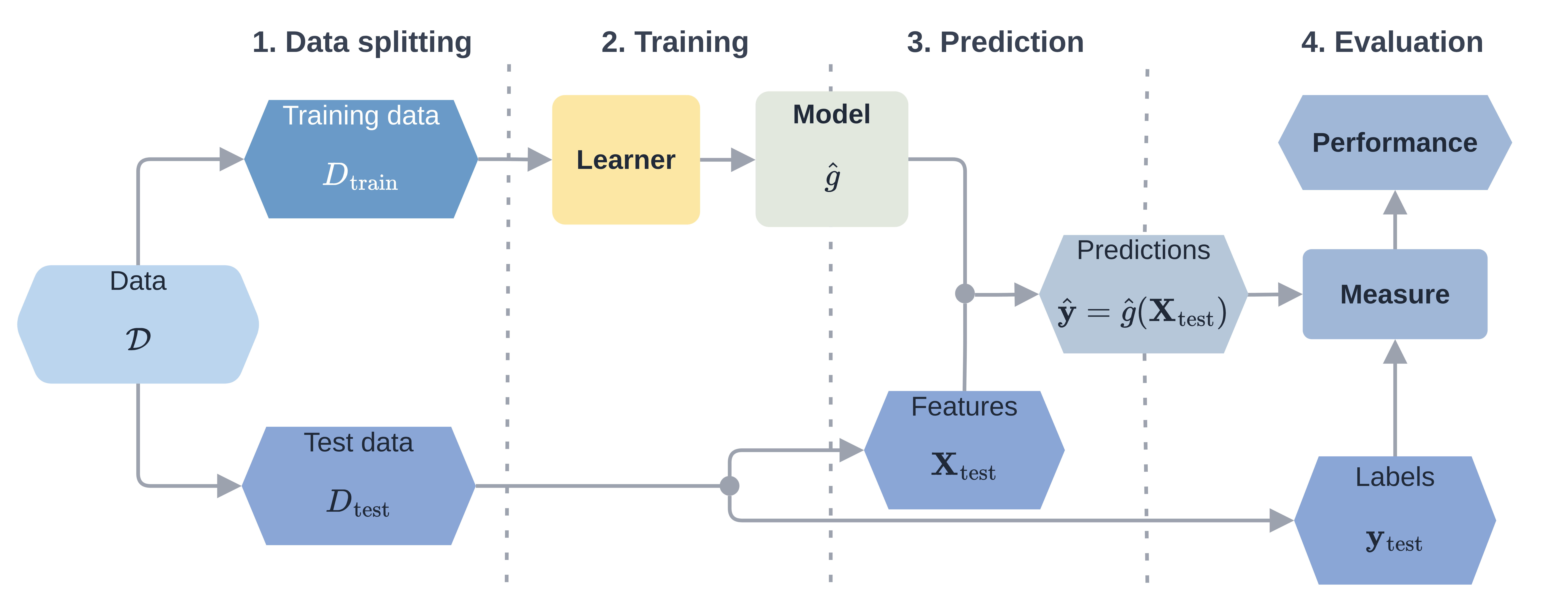
The basic machine learning workflow is represented in Figure 2.1:
- Data splitting: Data is split into training and test datasets.
- Training: A learner is selected and is trained on the training data, inducing a fitted model.
- Predicting: Features from the test data are passed to the model which makes predictions for the unseen outcomes (Box 1).
- Evaluation: Outcomes from the test data are passed to a chosen measure with the predictions, which evaluates the performance of the model (Box 2).
The process of (repeatedly) splitting the data into training and test data is called resampling and running multiple resampling experiments with different models is called benchmarking. All these concepts will be explained in this chapter.
2.2 Tasks
A machine learning task is the specification of the mathematical problem that is to be solved by a given algorithm. Tasks are derived from datasets and one dataset can give rise to many tasks. For example, a dataset with columns ‘age’, ‘weight’, ‘height’, ‘sex’, ‘diagnosis’, and ‘time of death’ could give rise to several supervised tasks:
- Supervised regression: Predict age from weight, height, and sex.
- Supervised classification: Predict sex from age and diagnosis.
- Supervised survival: Predict time of death from all other features.
The specification of a task is vital for interpreting predictions from a model and its subsequent performance. This is particularly true when separating between deterministic and probabilistic predictions, as discussed later in the chapter.
Formally, let \(\mathcal{X}\subseteq \mathbb{R}^p\) be the feature space for \(p\) features and let \(\mathcal{Y}\) be the target space (or outcomes or labels). A dataset is then given by \(\mathcal{D}= \{(\mathbf{x}_i, y_i)\}_{i=1}^n\) where the observations are assumed to be independent and identically distributed draws from an unknown joint distribution.
A machine learning task is the problem of learning the unknown function \(g : \mathcal{X}\rightarrow \mathcal{Y}\) where \(\mathcal{Y}\) specifies the nature of the task, for example classification, regression, or survival. For some tasks, the prediction object may differ from the outcome space, such as in probabilistic prediction tasks.
2.2.1 Regression
Regression tasks make continuous predictions, for example someone’s height. Regression may be deterministic, in which case a single continuous value is predicted, or probabilistic, where a probability distribution over the real numbers is predicted. For example, predicting an individual’s height as 165cm would be a deterministic regression prediction, whereas predicting their height follows a \(\mathcal{N}(165, 2^2)\) distribution would be probabilistic.
Formally, a deterministic regression task is specified by \(g_{Rd} : \mathcal{X}\rightarrow \mathcal{Y}\subseteq \mathbb{R}\), and a probabilistic regression task by \(g_{Rp} : \mathcal{X}\rightarrow \mathcal{S}\) where \(\mathcal{S}\subseteq \operatorname{Distr}(\mathcal{Y})\) and \(\operatorname{Distr}(\mathcal{Y})\) is the space of distributions over \(\mathcal{Y}\).
In the machine learning literature, deterministic regression is more common than probabilistic and hence the shorthand ‘regression’ is used to refer to deterministic regression.
2.2.2 Classification
Classification tasks make discrete predictions, for example whether it will rain, snow, or be sunny tomorrow. Similarly to regression, predictions may be deterministic or probabilistic. Deterministic classification predicts which category an observation falls into, whereas probabilistic classification predicts the probability of an observation falling into each category. Predicting it will rain tomorrow is a deterministic prediction whereas predicting \(\hat{p}(\text{rain}) = 0.6; \hat{p}(\text{snow}) = 0.1; \hat{p}(\text{sunny}) = 0.3\), is probabilistic.
Formally, a deterministic classification task is given by \(g_{Cd} : \mathcal{X}\rightarrow \mathcal{Y}\subseteq \mathbb{N}_0\), and a probabilistic classification task as \(g_{Cp} : \mathcal{X}\rightarrow [0,1]^k\) where \(k\) is the number of categories an observation may fall into and the predicted probabilities should sum to one. In practice, this latter prediction estimates the conditional class probabilities, \(\Pr(Y = y \mid X = \mathbf{x})\). If only two categories are possible, these reduce to the binary classification tasks: \(g_{Bd}: \mathcal{X}\rightarrow \{0, 1\}\) and \(g_{Bp}: \mathcal{X}\rightarrow [0, 1]\) for deterministic and probabilistic binary classification respectively.
In the probabilistic binary case it is common to formulate the task to predict \([0,1]\) not \([0,1]^2\) as the classes are mutually exclusive. The class for which probabilities are predicted is referred to as the positive class, and the other as the negative class.
2.3 Training and predicting
The terms algorithm, learner, and model are often conflated in machine learning. A learner is a description of a learning algorithm, prediction algorithm, parameters, and hyperparameters. The learning algorithm is a mathematical strategy to estimate the unknown mapping from features to outcome as represented by a task, \(g: \mathcal{X}\rightarrow \mathcal{Y}\). During training, data, \(\mathcal{D}\), is fed into the learning algorithm and induces the model \(\hat{g}\). Whereas the learner defines the algorithm for training and prediction, the model is the result of training the algorithm on data.
After training the model, a new observation, \(\mathbf{x}_*\), can be fed to the prediction algorithm, which is a mathematical strategy that uses the model to make a prediction, \(\hat{y}= \hat{g}(\mathbf{x}_*)\). Algorithms range in complexity from simple linear equations, with only a few coefficients to estimate, to complex iterative procedures whose training and prediction steps differ considerably.
Algorithms usually involve parameters and hyperparameters. Parameters are learned from data whereas hyperparameters are set beforehand to guide the algorithms. Model parameters (or weights), \(\boldsymbol{\theta}\), are coefficients to be estimated during model training. Hyperparameters, \(\boldsymbol{\lambda}\), control how the algorithms are run but are not directly updated by them. Hyperparameters can be mathematical, for example the learning rate in a gradient boosting machine (Chapter 14), or structural, for example the depth of a decision tree (Chapter 12) or the architecture of a neural network (Chapter 15). The number of hyperparameters usually increases with learner complexity and affects its predictive performance. Often hyperparameters need to be tuned (Section 2.5) instead of manually set.
An example bringing these concepts together is given in Box 1.
2.4 Evaluating and benchmarking
A central component of machine learning best practice is rigorous, empirical model evaluation. Building a complex model does not guarantee strong predictive performance. Moreover, testing performance on a single dataset only provides limited insight into how a model will generalize to new data. This issue is especially pronounced in modern pre-trained generative AI models, where there is often an implicit assumption by users that these models will perform well across a wide range of domains without task-specific validation. Trusting a model’s performance requires two elements: firstly, quantifying performance using appropriate and interpretable measures; secondly, clearly specifying what exactly is being assessed and how.
2.4.1 Evaluation
To understand whether a model is ‘good’, its predictions are evaluated with a loss function. In general, losses compare an observed outcome with a prediction object, which could be a numeric value, a class probability vector, or a predicted distribution. For deterministic predictions, loss functions assign a score to the discrepancy between predictions and true values, \(L: \mathcal{Y}\times \mathcal{Y}\rightarrow \bar{\mathbb{R}}\). This formulation is general and also covers losses that can take negative or infinite values, such as those based on the negative log-likelihood. In practice, many losses are non-negative, such as the absolute loss, \(L(y, \hat{y}) = \vert y - \hat{y} \vert\).
A model is considered truly useful if it performs well in general, meaning it should perform well on new, previously unseen data, rather than only the data encountered during training and development. A model’s generalization error refers to its expected performance on new data. Given some loss \(L\), a trained model \(\hat{g}\), and random data \((X, Y)\), then the generalization error is the expectation of the loss over an independent test sample, \(\mathbb{E}[L(Y, \hat{g}(X))]\).
A model should only be used to make predictions if its generalization error is estimated to be acceptable for a given context. If a model were trained and evaluated on the same data, the resulting loss, known as the training error, would be an overoptimistic estimate of the true generalization error (James et al. 2013). This occurs because the model is making predictions for data it has already ‘seen’ and therefore the loss does not evaluate the model’s ability to generalize to new, unseen data. Estimation of the generalization error requires data splitting, which is the process of splitting available data, \(\mathcal{D}\), into training data, \(\mathcal{D}_{train}\subset \mathcal{D}\), and testing data, \(\mathcal{D}_{test}= \mathcal{D}\setminus \mathcal{D}_{train}\). Another benefit of data splitting is to help detect model overfitting, which occurs when models learn patterns specific to the training data that do not generalize to new data. Overfitting can be mitigated through methods that constrain model complexity and reduce the tendency to fit noise in the training data; examples include feature selection, penalization methods, and early stopping.
2.4.2 Resampling and benchmarking
The simplest method to estimate the generalization error is holdout resampling, which is the process of partitioning the data into one training dataset and one testing dataset, with the model trained on the former and predictions made for the latter. Using 2/3 of the data for training and 1/3 for testing is a common splitting ratio (Kohavi 1995). Splitting the data randomly ensures that potential patterns or information encoded in the ordering of the data are removed; these patterns are unlikely to generalize to new, unseen data. For example, in clinical datasets, the order in which patients enter a study might inadvertently encode latent information such as which doctor was on duty at the time, which could theoretically influence patient outcomes. As this information is not explicitly captured in measured features, it is unlikely to hold predictive value for future patients. Random splitting breaks any spurious associations between the order of data and the outcomes.
Holdout resampling is a quick method to estimate the generalization error, and is particularly useful when very large datasets are available. However, holdout resampling has a very high variance for small datasets and there is no guarantee that evaluating the model on one holdout split is indicative of real-world performance.
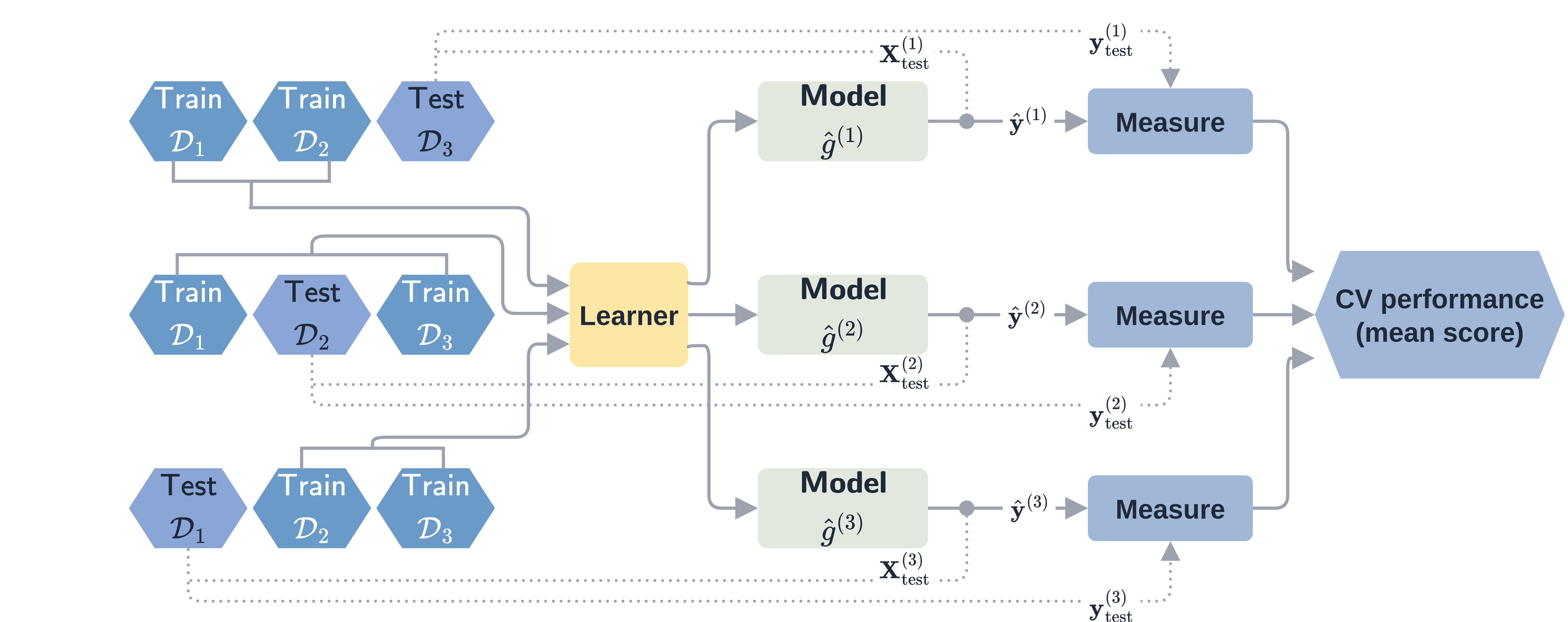
\(k\)-fold cross-validation (CV) can be used as a more robust method to estimate the generalization error (Hastie et al. 2001). \(k\)-fold CV partitions the data into \(k\) subsets, called folds. The training data consists of \(k-1\) of the folds and the remaining one is used for testing and evaluation. This is repeated \(k\) times until each of the folds has been used exactly once as the testing data. The performance from each fold is averaged into a final performance estimate (Figure 2.2). It is common to use \(k = 5\) or \(k = 10\) (Breiman and Spector 1992; Kohavi 1995). This process can be repeated multiple times (repeated \(k\)-fold CV) and/or \(k\) can even be set to \(n\), which is known as leave-one-out cross-validation.
Cross-validation can also be stratified, which ensures that a variable of interest will have the same distribution in each fold as in the original data. This is important, and often recommended, in survival analysis to ensure that the proportion of censoring in each fold is representative of the full dataset (Casalicchio and Burk 2024; Herrmann et al. 2021). Other resampling mechanisms may also be useful for event history analysis (Chapter 4). For example, stratifying with respect to different competing risks, or using more complex resampling schemes that can handle non-independent observations for recurrent events data (Hornung et al. 2023).
Repeating resampling experiments with multiple models is referred to as a benchmark experiment. A benchmark experiment compares models by evaluating their performance on identical data, which means the same resampling strategy and folds should be used for all models. Determining if one model performs better than another is a surprisingly complex topic (Benavoli et al. 2017; Demšar 2006; Dietterich 1998; Nadeau and Bengio 2003; Schulz-Kümpel et al. 2025) and is out of scope for this book. A common heuristic is to suggest one model outperforms another if it consistently performs better across the majority of folds in a repeated cross-validation benchmark experiment. However, this is just a heuristic and without robust hypothesis testing results should be interpreted with caution.
2.5 Hyperparameter optimization
Section 2.3 introduced model hyperparameters, which control how training and prediction algorithms are run. Setting hyperparameters is a critical part of model fitting and can significantly change model performance. Tuning is the process of using internal benchmark experiments to automatically select the optimal hyperparameter configuration. For example, the regularization parameter, \(\gamma\), in ridge regression is a potential hyperparameter to tune. This hyperparameter may be tuned over a range of values, say \([0.1, 25]\), or over a discrete subset, for example \(\{0.1, 10, 25\}\). Using the discrete example, tuning the regularization parameter would effectively involve comparing three independent ridge regression models in a benchmark experiment with \(\gamma=0.1\), \(\gamma=10\), and \(\gamma=25\) respectively. The value of \(\gamma\) that results in the model with the optimal performance is then selected for the hyperparameter value going forward. Nested resampling is a method to reduce bias that could occur from using overlapping data for tuning, training, or testing (Simon 2007). Nested resampling is the process of resampling the training set again for tuning before then refitting the optimal model on the entire training data.
2.6 Parameter optimization
Many machine learning models, including gradient boosting machines (Chapter 14) and neural networks (Chapter 15), depend on iteration to fit parameters to the training data. This section briefly covers a common technique for iterative parameter optimization using gradient descent (Section 2.6.1) and then a process for controlling the number of iterations known as early stopping (Section 2.6.2).
2.6.1 Gradient descent
Many machine learning algorithms use gradient descent to estimate the model parameters, \(\boldsymbol{\theta}\), during training. Gradient descent is commonly used when no closed-form solution exists for minimizing a loss function. Given a differentiable loss function, \(L(\boldsymbol{\theta})\), that measures how well the model predicts the training data, gradient descent repeatedly updates the parameter estimates by taking small steps that decrease the loss until the loss stabilizes or a stopping criterion is met. This principle is central to neural networks (Chapter 15) and is closely related to the functional gradient view of gradient boosting (Chapter 14), but is easier to introduce for a simple linear regression model with only two parameters.
Consider the linear regression model \(y = g(x \mid \boldsymbol{\theta}) = \beta_0 + \beta_1 x\) with parameter vector \(\boldsymbol{\theta}= (\beta_0 \ \beta_1)^\top\), fitted to observations \(\{(x_i, y_i)\}^n_{i=1}\) by minimizing the mean squared error loss:
\[ L(\boldsymbol{\theta}) = \frac{1}{n}\sum_{i=1}^n \bigl(y_i - \beta_0 - \beta_1 x_i\bigr)^2. \tag{2.1}\]
The gradient of this loss is the vector of partial derivatives of the loss with respect to each parameter:
\[ \nabla_{\boldsymbol{\theta}} L = \bigl(\partial L / \partial \beta_0 \ \partial L / \partial \beta_1\bigr)^\top. \]
For any parameter values \(\boldsymbol{\theta}\), the gradient describes how the loss changes when the parameters are changed. If the gradient component for a parameter is positive, decreasing that parameter reduces the loss; if negative, increasing the parameter reduces the loss. Gradient descent therefore updates the parameters in the opposite direction of the gradient to reduce the loss, \[ \boldsymbol{\theta}^{t+1} = \boldsymbol{\theta}^{t} - \alpha \,\nabla_{\boldsymbol{\theta}} L\bigl(\boldsymbol{\theta}^{t}\bigr), \tag{2.2}\]
where \(\alpha > 0\) is the learning rate, also known as the step size, as it controls the size of the parameter update at each iteration. If \(\alpha\) is too small, then convergence is slow, but if it is too large, iterations can overshoot or oscillate. In machine learning models \(\alpha\) is typically tuned (Section 2.5) or adaptive and combined with early stopping (Section 2.6.2).
Starting from an arbitrary initial guess \(\boldsymbol{\theta}^{0}\), (2.2) is repeated to drive \(\boldsymbol{\theta}\) towards a minimum of \(L\).
For the loss in (2.1), the partial derivatives are: \[ \begin{aligned} \frac{\partial L}{\partial \beta_0} &= -\frac{2}{n}\sum_{i=1}^n (y_i - \beta_0 - \beta_1 x_i), \\ \frac{\partial L}{\partial \beta_1} &= -\frac{2}{n}\sum_{i=1}^n x_i (y_i - \beta_0 - \beta_1 x_i). \end{aligned} \tag{2.3}\]
In a simple example, suppose the data are \(\{(3, 1.8), (2, 14)\}\), the initial guess is \(\boldsymbol{\theta}^{0} = (1 \ 1)^\top\), and \(\alpha=0.1\), then substituting (2.3) into (2.2) gives:
\[ \begin{aligned} \boldsymbol{\theta}^1 &= \begin{pmatrix} 1 \\ 1 \\ \end{pmatrix} - 0.1 \begin{pmatrix} -\frac{2}{n}\sum_{i=1}^n (y_i - 1 - x_i) \\ -\frac{2}{n}\sum_{i=1}^n x_i (y_i - 1 - x_i) \\ \end{pmatrix} \\ &= \begin{pmatrix} 1 \\ 1 \\ \end{pmatrix} - 0.1 \begin{pmatrix} -\frac{2}{2}((1.8 - 1 - 3) + (14 - 1 - 2)) \\ -\frac{2}{2}(3(1.8 - 1 - 3) + 2(14 - 1 - 2)) \\ \end{pmatrix} \\ &= \begin{pmatrix} 1 \\ 1 \\ \end{pmatrix} - 0.1 \begin{pmatrix} -8.8 \\ -15.4 \\ \end{pmatrix} = \begin{pmatrix} 1.88 \\ 2.54 \\ \end{pmatrix}. \end{aligned} \]
As can be seen, each gradient-descent step updates all parameters simultaneously.
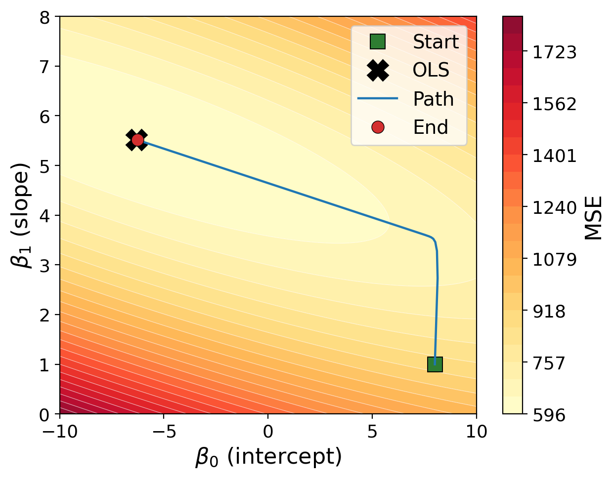
Linear regression minimized by the mean squared error has a known, closed-form solution (ordinary least squares). Figure 2.3 illustrates gradient descent for an example with more observations, comparing the gradient descent procedure to the known closed-form optimum. The contours show the loss surface of \(L(\boldsymbol{\theta})\) over the two-dimensional parameter space; lighter colors correspond to a smaller loss. Starting from a deliberately poor initial guess (green square), gradient descent traces the blue path along the loss surface and finishes (red circle) at the known closed-form optimum (black cross). At every step, the update moves in the direction \(-\nabla_{\boldsymbol{\theta}} L\); as the gradient becomes smaller near the optimum, the parameter updates also become smaller.
Adaptations to gradient descent, including stochastic gradient descent and mini-batching, are discussed in Section 15.1.2.1.
2.6.2 Early stopping
Iterative optimization introduces a practical question: how many iterations should be used? Continuing training for too long can lead to overfitting in which the model starts to capture noise specific to the training data and generalizes poorly to new observations. The number of iterations is therefore a hyperparameter controlling model complexity. Instead of tuning this hyperparameter, a common technique is to use early stopping.
Early stopping monitors predictive performance on a held-out validation set (Section 2.4.2) as training proceeds. This validation set is typically a subset of the training dataset, meaning that it is common for a dataset \(\mathcal{D}\) to be split into \(\mathcal{D}_{train}\) for training the model, \(\mathcal{D}_{validation}\) for monitoring performance during training, and \(\mathcal{D}_{test}\) for evaluating performance after training. These datasets can be created using any of the resampling methods in Section 2.4.2. As discussed in Section 2.4.1, evaluating a model on the training data results in overoptimistic estimates of the true generalization error. As the number of iterations increases, the training error decreases steadily, whereas the validation error typically decreases at first and then begins to increase once the model starts to overfit. Figure 2.4 illustrates this on the gradient-descent example of Section 2.6.1, using part of the data for training and the remainder for validation.
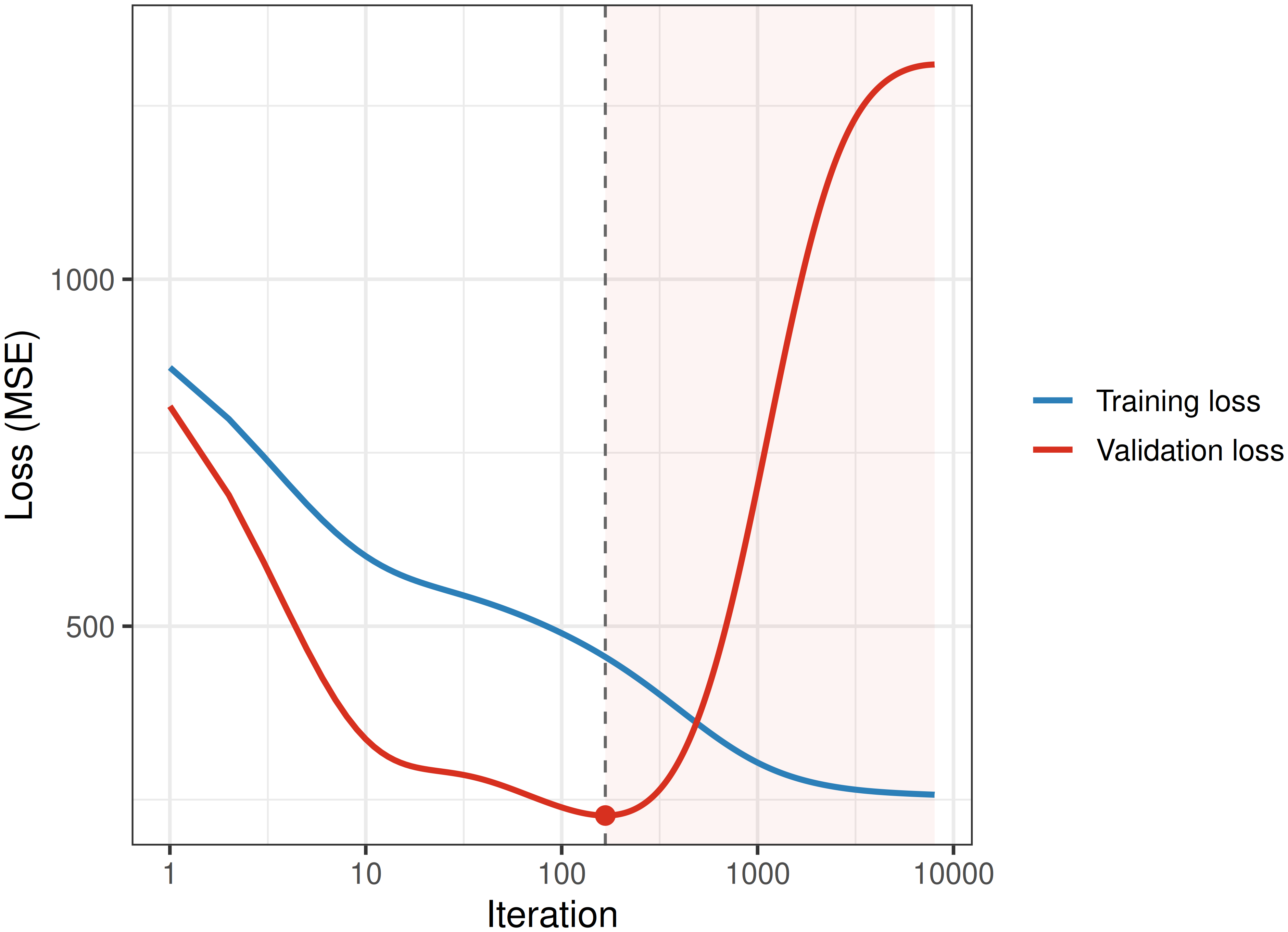
Theoretically, training could be stopped as soon as the validation loss starts to increase, visualized by the red point in Figure 2.4. However, the validation loss rarely improves smoothly from one iteration to the next, so a patience hyperparameter is used, which is the number of consecutive iterations in which the validation loss must fail to improve before stopping the training algorithm. Early stopping is computationally cheaper than tuning the number of iterations directly (Section 2.5), which would require repeatedly fitting complete models. Early stopping can also be viewed as a form of regularization, as limiting the number of iterations restricts how closely the model can fit the training data, in a similar spirit to how shrinkage or penalty terms constrain model complexity.