12 Random Forests
Random forests are a composite (or ensemble) algorithm built by fitting many simpler component models, decision trees, and then averaging their predictions. Due to their built-in feature selection capabilities, random forests are commonly used in high-dimensional settings when the number of variables far exceeds the number of observations (rows). Despite being black boxes, especially as the number of trees increases, random forests have natural feature importance measures which make them one of the more interpretable machine learning algorithms. Random survival forests therefore remain a popular and well-performing model in the survival setting, both for predictive modeling and pattern recognition.
12.1 Random forests for regression
Training of decision trees can include a large number of hyperparameters and different training steps including ‘growing’ and subsequently ‘pruning’. However, when utilized in random forests, many of these parameters and steps can be safely ignored, hence this section only focuses on the components that primarily influence the resulting random forest. This section will start by discussing decision trees and will then introduce the bagging algorithm used to create random forests.
12.1.1 Decision trees
Decision trees are machine learning models that are comparatively simple to implement in software and are highly interpretable. A decision tree algorithm takes a dataset as input and partitions the data into distinct, non-overlapping subsets known as nodes. Partitioning is performed by applying a splitting rule to a single feature, creating branches that divide the data according to a selected cutoff or category. This process is repeated recursively, potentially using different features at each split, until a stopping rule is reached. The final nodes are referred to as terminal nodes or leaves.
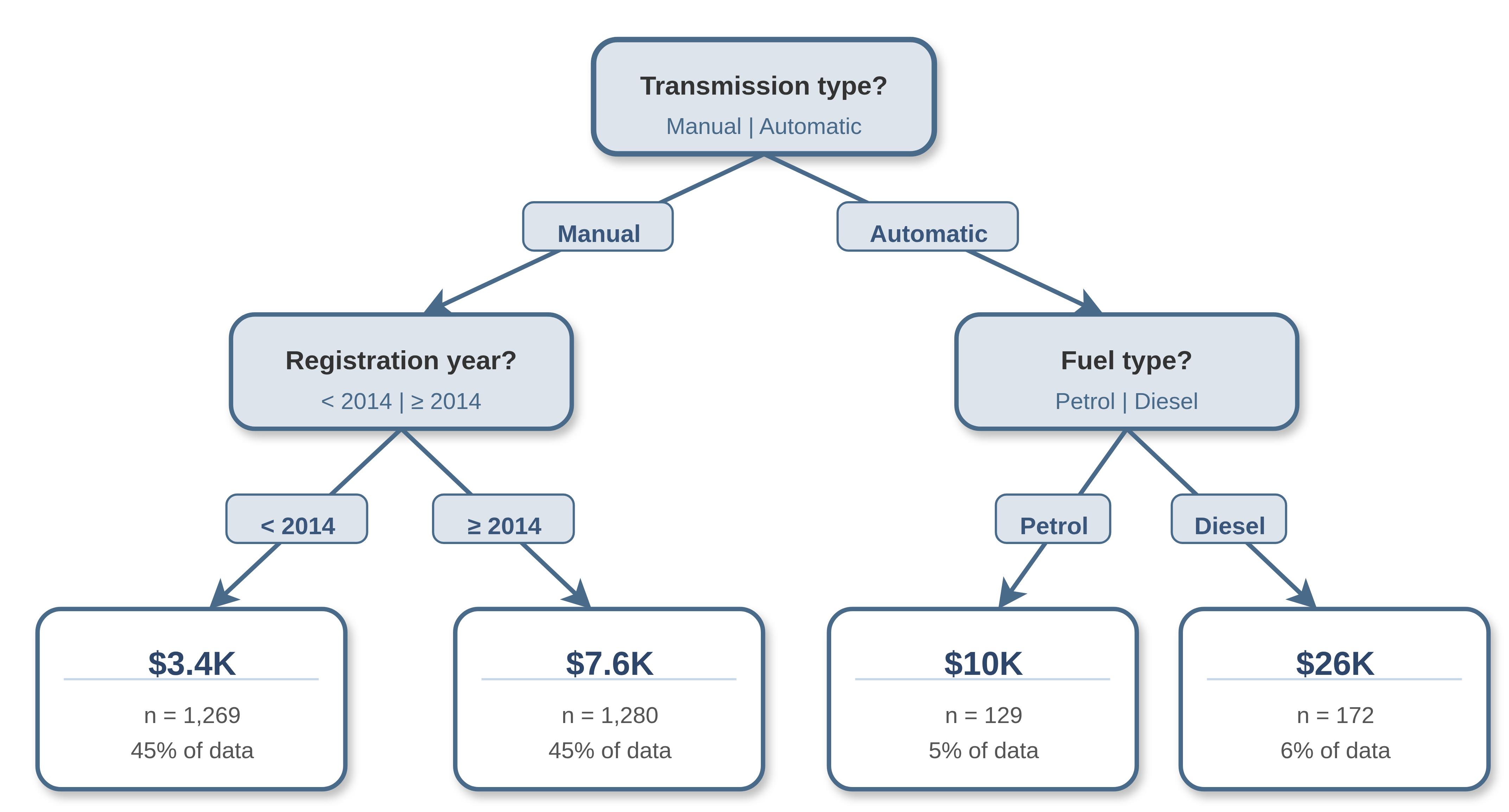
For example, (Figure 12.1) demonstrates a decision tree predicting the price that a car sells for in India (price in thousands of dollars). The dataset includes as variables: transmission type (manual or automatic), registration year, fuel type (petrol or diesel), number of owners, kilometers driven, and seller type. The decision tree was trained with a maximum depth of 2 (the number of rows excluding the top), and it can be seen that with this restriction only the transmission type, registration year, and fuel type were selected variables. During training, the algorithm identified that the first optimal variable to split the data was transmission type, partitioning the data into manual and automatic cars. Manual cars are further split by registration year whereas automatic cars are split by fuel type. The average sale prices in the final leaves are the terminal node predictions (Section 12.1.1.2).
The graphic highlights several core features of decision trees:
- they can model non-linear and interaction effects: The hierarchical structure allows for complex interactions between variables with some variables being used to separate all observations (transmission) and others only applied to subsets (year and fuel);
- they are highly interpretable: it is easy to visualize the tree and see how predictions are made;
- they perform variable selection: not all variables were used to train the model.
To understand how random forests work, it is worth looking a bit more into the most important components of decision trees: splitting rules, stopping rules, and terminal node predictions.
12.1.1.1 Splitting and stopping rules
Precisely how the data partitions/splits are derived and which variables are utilized is determined by the splitting rule. The goal in each partition is to find two resulting nodes that have the greatest difference between them and thus the maximal homogeneity within each node. Hence, after each split, the data in each node should become increasingly similar. The splitting rule provides a way to measure the difference between nodes or the homogeneity within the resulting nodes. In regression, the most common splitting rule is to select a variable and cutoff (a threshold on the variable at which to separate observations) that minimizes the mean squared error in the two potential resulting nodes.
For all decision tree and random forest algorithms going forward, let \(\mathcal{A}\) denote the set of observation indices in a node, with mean outcome:
\[ \bar{y}_{\mathcal{A}} = \frac{1}{\vert \mathcal{A} \vert}\sum_{i \in \mathcal{A}} y_i. \]
Let \(j = 1,\ldots,p\) index the features and let \(c_j\) be a possible cutoff value for feature \(j\). For parent node \(\mathcal{A}\), define:
\[ \begin{aligned} &\mathcal{A}^l(j,c_j) := \{i \in \mathcal{A}: x_{i,j} < c_j\}, \\ &\mathcal{A}^r(j,c_j) := \{i \in \mathcal{A}: x_{i,j} \geq c_j\}, \end{aligned} \]
as the two nodes resulting from partitioning feature \(j\) at cutoff \(c_j\). To simplify notation, let \(\mathcal{A}^l, \mathcal{A}^r\) denote \(\mathcal{A}^l(j,c_j)\) and \(\mathcal{A}^r(j,c_j)\) respectively. The optimal split is determined by the arguments \((j^*, c^*_{j^*})\) that minimize the residual sum of squares across both nodes (James et al. 2013),
\[ (j^*, c_{j^*}^*) = \mathop{\mathrm{arg\,min}}_{j, c_j} \sum_{i \in \mathcal{A}^l} (y_i - \bar{y}_{\mathcal{A}^l})^2 + \sum_{i \in \mathcal{A}^r} (y_i - \bar{y}_{\mathcal{A}^r})^2. \]
This method is repeated from the first node to the last such that observations are included in a given node \(\mathcal{A}\) if they satisfy all conditions from all previous branches (splits); features may be considered multiple times in the growing process allowing complex interaction effects to be captured.
Nodes are repeatedly split until a stopping rule has been triggered — a criterion that tells the algorithm to stop partitioning data. The stopping rule is usually a condition on the number of observations in each node such that nodes will continue to be split until some minimum number of observations has been reached in a node. Other conditions may be on the depth of the tree (as in Figure 12.1 which is restricted to a maximum depth of 2), which corresponds to the number of levels of splitting. Stopping rules are often used together, for example by setting a maximum tree depth and prespecifying a minimum number of observations per leaf. Deciding the minimum number of observations and/or the maximum depth can be performed with tuning (Section 2.5).
12.1.1.2 Terminal node predictions
The final major component of decision trees is terminal node predictions. As the name suggests, this is the part of the algorithm that determines how to actually make a prediction for a new observation. A prediction is made by ‘dropping’ the new data ‘down’ the tree according to the optimal splits that were found during training. The resulting prediction is then a simple baseline statistic computed from the training data in the corresponding node. In regression, this is commonly the sample mean of the training outcome data.
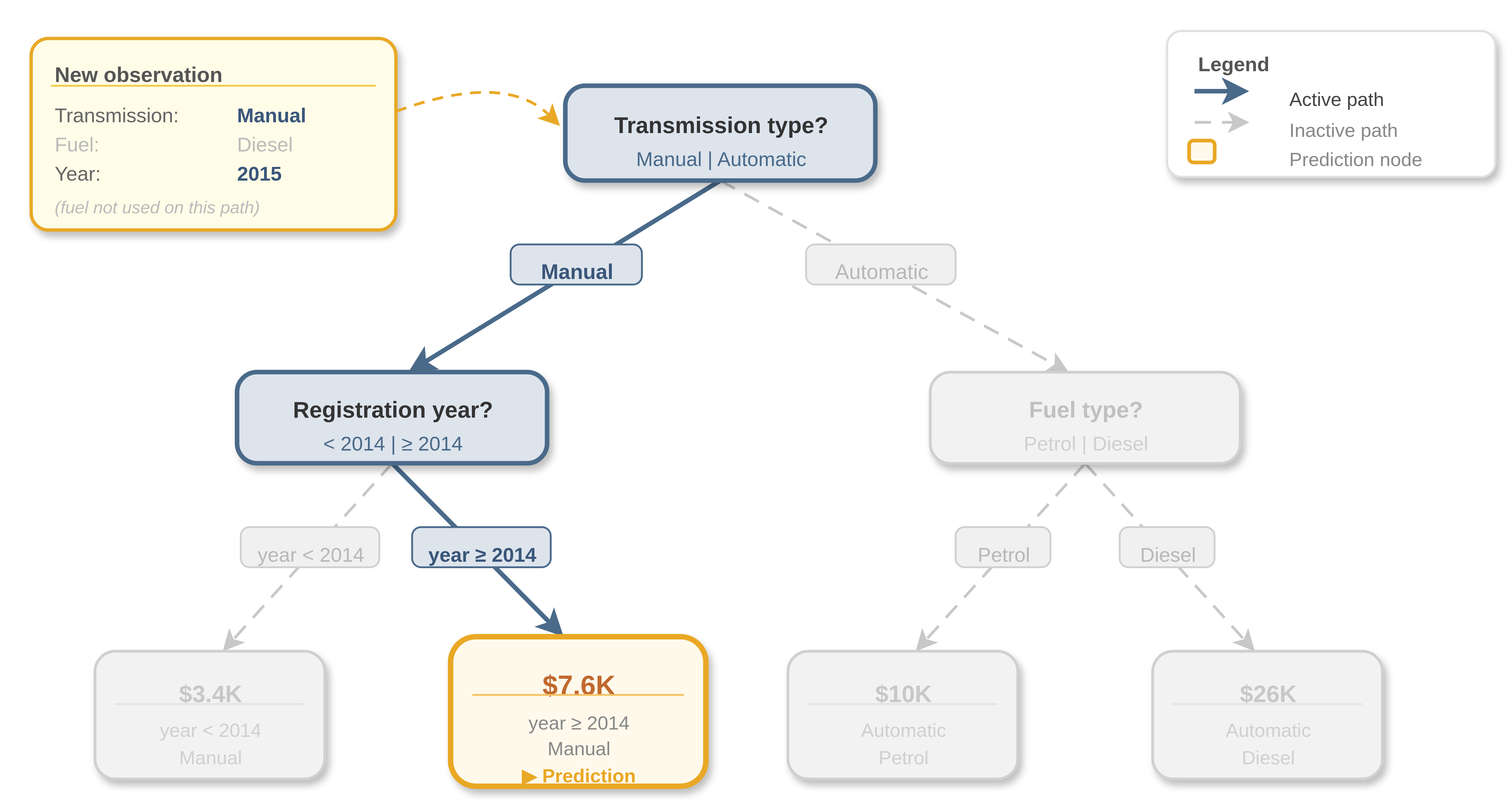
Returning to Figure 12.1, say a new data point is {transmission = Manual, fuel = Diesel, year = 2015}, then in the first split the left branch is taken as ‘transmission = Manual’, in the second split the right branch is taken as ‘year’ \(= 2015 \geq 2014\), hence the new data point lands in the second terminal leaf and is predicted to sell for \(7,600\). The ‘fuel’ variable is ignored as it is only considered for automatic vehicles. Figure 12.2 illustrates this prediction path through the tree. This also highlights another powerful feature of random forests: as the final predictions are simple statistics based on training data, all potential predictions can be saved in the original trained model and no complex computations are required in the prediction algorithm.
12.1.2 Random forests
Decision trees often overfit the training data, hence they have high variance, perform poorly on new data, and are not robust to even small changes in the original training data. Moreover, important variables can end up being ignored as only subsets of dominant variables are selected for splitting.
Random forests treat individual decision trees as high-variance base learners. Each tree may be unstable on its own, but averaging predictions over many decorrelated trees produces a more stable predictor. Random forests utilize bootstrap aggregation, or bagging (Breiman 1996), to aggregate many decision trees as follows:
- for \(b = 1,\ldots,B\):
- \(D_b \gets \text{ Randomly sample with replacement from } \mathcal{D}_{train}\)
- \(\hat{g}_b \gets \text{ Train a decision tree on } D_b\)
- end for
- return \(\{\hat{g}_b\}^B_{b=1}\)
Step 2 is known as bootstrapping, which is the process of sampling a dataset with replacement. In random forest implementations this is more common than standard subsampling where data is sampled without replacement. Commonly, the bootstrapped sample size is the same as the original. However, as the same value may be sampled multiple times, on average the resulting data only contains around 63.2% unique observations (Efron and Tibshirani 1997). Randomness is further injected to decorrelate the trees by randomly subsetting the candidates of features to consider at each split of a tree. Therefore, every split of every tree may consider a different subset of variables. This process is repeated for \(B\) trees, with the final output being a collection of trained decision trees. The number of trees is a hyperparameter, but in practice \(B\) is usually chosen to be large, with an early stopping-type procedure (Section 2.6.2) used to grow trees until validation performance stabilizes. Beyond this point, additional trees mainly increase computational cost while providing diminishing improvements in predictive performance.
Prediction from a random forest for new data \(\mathbf{x}_*\) follows by making predictions from the individual trees and aggregating the results by some function \(\sigma\), which is usually the sample mean for regression:
\[ \hat{g}(\mathbf{x}_*) = \sigma(\hat{g}_1(\mathbf{x}_*),\ldots,\hat{g}_B(\mathbf{x}_*)) = \frac{1}{B} \sum^B_{b=1} \hat{g}_b(\mathbf{x}_*) \]
where \(\hat{g}_b(\mathbf{x}_*)\) is the prediction from the \(b\)th tree for some new data \(\mathbf{x}_*\) and \(B\) is the total number of grown trees.
As discussed above, individual decision trees result in predictions with high variance that are not robust to small changes in the underlying data. Random forests decrease this variance by aggregating predictions over a large sample of decorrelated trees, where a high degree of difference between trees is promoted through the use of bootstrapped samples and random candidate feature selection at each split.
Usually many (hundreds or thousands) trees are grown, which makes random forests robust to changes in data with more stable predictions. Other advantages include having tunable and meaningful hyperparameters, including: the number of variables to consider for a single split, the splitting rule, and the stopping rule.
While random forests are considered a black box, in that one cannot be reasonably expected to inspect thousands of individual trees, variable importance can still be aggregated across trees, for example by counting the frequency a variable was selected across trees, calculating the minimal depth at which a variable was used for splitting, or via permutation-based feature importance. Hence random forest models are usually more interpretable than many alternative methods. Finally, random forests are less prone to overfitting than individual trees as predictions are averaged across many decorrelated trees.
12.2 Random survival forests
Random forests can be adapted to random survival forests by updating the splitting rules and terminal node predictions to those that can handle censoring and can make survival predictions. This chapter is therefore focused on outlining different choices of splitting rules and terminal node predictions, which can then be flexibly combined into different models.
12.2.1 Splitting rules
Survival trees and random survival forests (RSFs) have been studied for the past four decades and while there are many possible splitting rules (Bou-Hamad et al. 2011), only two broad classes are commonly utilized (as judged by number of available implementations, for example, Ishwaran et al. 2011; Pölsterl 2020; Wright and Ziegler 2017). The first class relies on the log-rank test to maximize dissimilarity between splits, the second class utilizes likelihood-based measures. The first is discussed in more detail as this is common in practice and is relatively straightforward to implement and understand. Likelihood rules are more complex and may require assumptions that are not realistic, these are discussed briefly.
12.2.1.1 Log-rank test
The log-rank test statistic has been widely utilized as a splitting rule for survival analysis (Ciampi et al. 1986; Ishwaran et al. 2008; LeBlanc and Crowley 1993; Segal 1988). The log-rank test compares the survival distributions of two groups under the null hypothesis that both groups have the same underlying risk of (immediate) events, with the hazard function used to compare underlying risk.
Let \(\mathcal{A}^l\) and \(\mathcal{A}^r\) be two nodes, and as before \(i \in \mathcal{A}\) indexes the observations in node \(\mathcal{A}\). Define:
\(n_\tau^l\), the number of observations at risk at time point \(\tau\) in node \(\mathcal{A}^l\) \[ n_\tau^l = \sum_{i \in \mathcal{A}^l} \mathbb{I}(t_i \geq \tau); \]
\(o^l_{\tau}\), the observed number of events at time point \(\tau\) in node \(\mathcal{A}^l\)
\[ o^l_{\tau} = \sum_{i \in \mathcal{A}^l} \mathbb{I}(t_i = \tau, \delta_i = 1); \]
- \(n_\tau = n_\tau^l + n_\tau^r\), the number of observations at risk at \(\tau\) in both nodes;
- \(o_\tau = o^l_{\tau} + o^r_{\tau}\), the observed number of events at \(\tau\) in both nodes.
Recall \(t_{(k)}\) is the \(k\)th ordered event time. The log-rank test evaluates if hazard functions are equal in both nodes, \(H_0: h^l = h^r\), with test statistic (Segal 1988),
\[ LR(\mathcal{A}^l) = \frac{\sum_{k=1}^m (o^l_{t_{(k)}} - e^l_{t_{(k)}})}{\sqrt{\sum_{k=1}^m v_{t_{(k)}}^l}}, \]
where:
- \(e^l_{\tau}\) is the expected number of events in node \(\mathcal{A}^l\) at \(\tau\):
\[ e^l_{\tau} := o_\tau\frac{n_\tau^l}{n_\tau}; \]
- \(v^l_\tau\) is the variance of the number of events in node \(\mathcal{A}^l\) at \(\tau\):
\[ v^l_{\tau} := e^l_{\tau} \Big(\frac{n_\tau - o_\tau}{n_\tau}\Big)\Big(\frac{n_\tau - n^l_\tau}{n_\tau - 1}\Big). \]
These results follow from the assumption that, under equal hazards in both nodes, the number of events at each unique event time follows a hypergeometric distribution. Under \(H_0\), \(LR(\mathcal{A}^l)^2\) follows a \(\chi^2\) distribution with one degree of freedom and the log-rank statistic is commonly reported alongside its corresponding \(p\)-value. In the two group setting, \(LR(\mathcal{A}^l) = -LR(\mathcal{A}^r)\), hence it is sufficient to compute the statistic for only one of the two nodes.
The higher the (absolute) log-rank statistic, the greater the dissimilarity between the two groups (Figure 12.3), thereby making it a sensible splitting rule for random forests; it has also been shown that it works well for splitting censored data (LeBlanc and Crowley 1993). Additionally, the log-rank test requires no knowledge about the shape of the survival curves or distribution of the outcomes in either group (Bland and Altman 2004), making it ideal for an automated process that requires no user intervention.
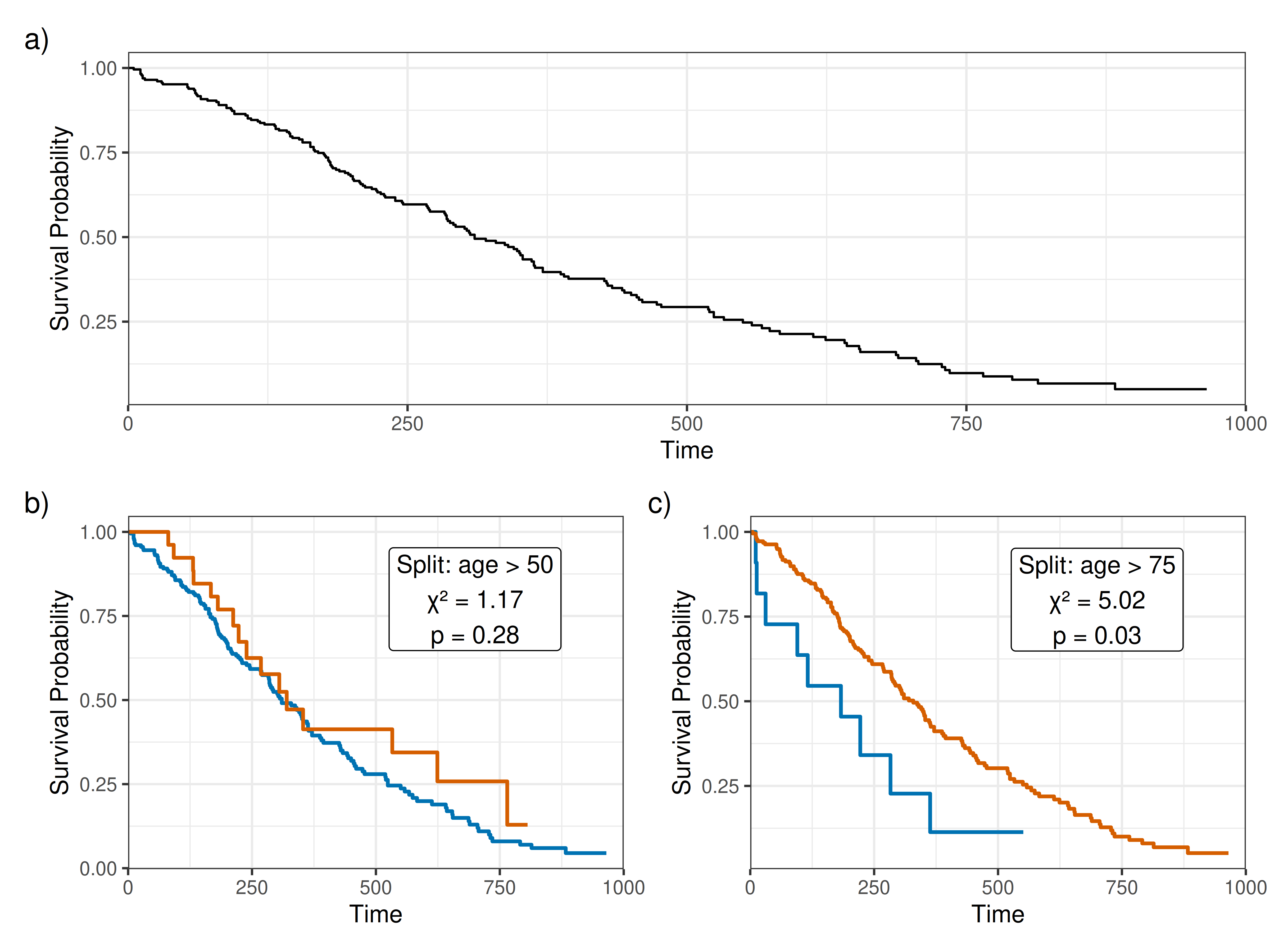
lung dataset from the \(\textsf{R}\) package survival. (b-c) is the same data stratified according to whether ‘age’ is greater or less than 50 (panel b) or 75 (panel c). The higher \(\chi^2\) statistic (panel c) results in a lower \(p\)-value and a greater difference between the stratified Kaplan-Meier curves. Therefore, splitting age at 75 results in a greater dissimilarity between the resulting branches and thus makes a better choice for splitting the variable.
The log-rank score rule (Hothorn and Lausen 2003) is a standardized version of the log-rank rule that could be considered as a splitting rule, though simulation studies have not demonstrated significant improvements in predictive performance when comparing the two (Ishwaran et al. 2008). Alternative dissimilarity measures and tests have also been suggested as splitting rules, including modified Kolmogorov-Smirnov test and Gehan-Wilcoxon tests (Ciampi et al. 1988). Simulation studies have demonstrated that both of these may have higher power and produce ‘better’ results than the log-rank statistic (Fleming et al. 1980), however neither appears to be commonly used.
12.2.1.2 Alternative splitting rules
A splitting rule is simply a way to measure if average performance across resulting nodes increases after data splitting. Therefore, there are many statistics that could be used for this purpose (Gordon and Olshen 1985; Ishwaran and Kogalur 2018; Schmid et al. 2016), including many of the metrics referenced in Part II. Like many other aspects of modeling, experiments have shown that the choice of splitting rules is data dependent (Schmid et al. 2016). When using loss-based splitting rules, a sensible approach is to align the splitting rule with the prediction problem. The log-rank splitting rule is commonly used when the goal is to maximize homogeneity within each node; for example, to most accurately estimate the within-node survival distribution. However, if the goal were to optimize the ranking of observations, then a concordance splitting rule may be optimal (Section 6.1).
An alternative to log-rank statistics and loss-based splitting rules is to instead use likelihood ratio, or deviance, statistics (LeBlanc and Crowley 1992). The likelihood-ratio statistic evaluates whether model fit improves after a candidate split and can therefore be used as a natural splitting rule. An advantage of likelihood-based methods is that alternative censoring mechanisms and truncation can be incorporated naturally through the likelihood formulation (3.15). However, specifying an appropriate parametric form for each fit is non-trivial, and assumptions that poorly reflect the data may lead to inferior splits. In principle, likelihood-based splitting rules may yield trees that better fit the data. Random forests are built from many base learners whose predictions are stabilized through averaging, so optimizing the fit of each individual tree may be unnecessary and any gains may be outweighed by sensitivity to model assumptions. Moreover, likelihood-based methods are implemented in relatively few off-the-shelf software packages and there is limited research formally comparing them with alternative splitting rules.
12.2.2 Terminal node prediction
Similarly to the regression setting, RSF predictions are typically based on simple estimates computed from the training data that fall within the terminal nodes. As seen throughout this book, the choice of estimator in the survival setting depends on the prediction task of interest. This section focuses on probabilistic predictions for the single-event setting, extensions to competing risks are discussed in Section 12.2.3, and then relative risk predictions for both settings are described in Section 12.2.4.
Terminal node predictions are only useful when there are sufficient uncensored observations in each terminal node. Hence, a common RSF stopping rule is to set a threshold on the minimum number of uncensored observations per node, meaning that a node is not split if doing so would result in too few uncensored observations to make meaningful predictions. When the minimum uncensored node size is not exposed as a hyperparameter, it can be tuned indirectly through the standard minimum node size. Alternatively, a useful heuristic is to take the recommended default minimum node size and divide it by the uncensored proportion in the data. For example, if the default minimum node size is \(10\) and \(30\%\) of the data are censored, then the adjusted minimum node size is \(\lceil 10/0.7 \rceil = 15\).
For survival distribution predictions, the algorithm requires a simple estimate for the underlying survival distribution in each of the terminal nodes, which can be estimated using the Kaplan-Meier (3.19) or Nelson-Aalen (3.21) estimators (Hothorn et al. 2004; Ishwaran et al. 2008; LeBlanc and Crowley 1993; Segal 1988).
Let \(b \in \{1,\ldots,B\}\) index the trees in a forest, let \(\mathcal{A}_b(\mathbf{x}_*)\) denote the terminal node in tree \(b\) that observation \(\mathbf{x}_*\) falls into, and let \(t^*_{(1)} < \ldots < t^*_{(m)}\) be the ordered event times within \(\mathcal{A}_b(\mathbf{x}_*)\). Then the predicted survival function and cumulative hazard for \(\mathbf{x}_*\) are,
\[ \hat{S}_{b}(\tau \mid \mathbf{x}_*) = \prod_{k:t^*_{(k)} \leq \tau} \left(1-\frac{d_{t^*_{(k)}}}{n_{t^*_{(k)}}}\right), \tag{12.1}\]
and,
\[ \hat{H}_{b}(\tau \mid \mathbf{x}_*) = \sum_{k:t^*_{(k)} \leq \tau} \frac{d_{t^*_{(k)}}}{n_{t^*_{(k)}}}, \tag{12.2}\]
where \(d_{t^*_{(k)}}\) and \(n_{t^*_{(k)}}\) are the observed number of events and the number of observations at risk at \(t^*_{(k)}\), both computed from observations in \(\mathcal{A}_b(\mathbf{x}_*)\). Direct calculation of the cumulative hazard using (12.2) avoids \(\log(0)\) errors which could occur if transforming from the Kaplan-Meier estimates in (12.1). See Figure 12.4 for an example using the lung dataset (Therneau 2024).
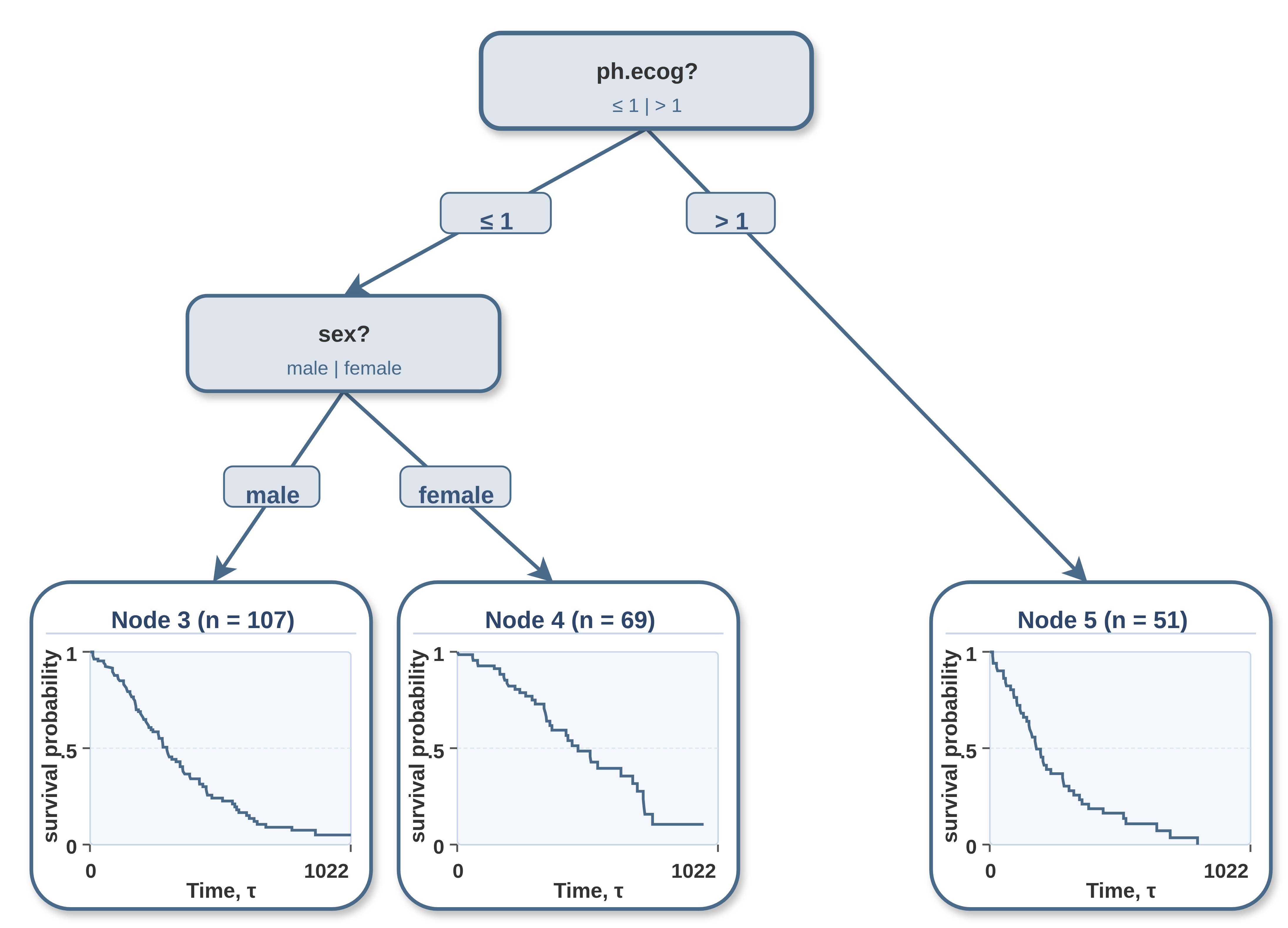
lung dataset from the \(\textsf{R}\) package survival. The terminal node predictions are survival curves.
The bootstrapped prediction may be formed either by averaging survival or cumulative hazard functions over individual trees. By definition, a mixture of \(n\) distributions with cumulative distribution functions \(F_i, i = 1,\ldots,n\) is given by,
\[ F(x) = \sum^n_{i=1} w_i F_i(x), \]
for some weights \(w_i, i = 1, \ldots, n\). Substituting \(F = 1 - S\) and noting \(\sum w_i = 1\) gives the computation \(S(x) = \sum^n_{i=1} w_i S_i(x)\), allowing the bootstrapped survival function to exactly represent the mixture distribution defined by the tree-specific survival functions:
\[ \hat{S}_{Boot}(\tau \mid \mathbf{x}_*) = \sum^B_{b=1} w_b\hat{S}_b(\tau \mid \mathbf{x}_*), \tag{12.3}\]
usually with \(w_b = 1/B\) where \(B\) is the number of trees. Alternatively, an ensemble estimator can be taken over the cumulative hazards:
\[ \hat{H}_{Boot}(\tau \mid \mathbf{x}_*) = \sum^B_{b=1} w_b\hat{H}_b(\tau \mid \mathbf{x}_*). \tag{12.4}\]
The cumulative hazard ensemble (12.4) does not generally correspond to the cumulative hazard of a mixture distribution, since \(\hat{S}_{Boot}(\tau \mid \mathbf{x}_*) \ne \exp(-\hat{H}_{Boot}(\tau \mid \mathbf{x}_*))\), though this does not affect its validity as an ensemble estimator.
In other censoring and truncation settings, the estimator in the final node can be replaced by the non-parametric maximum likelihood estimator or left-truncated risk set (Section 3.5.2).
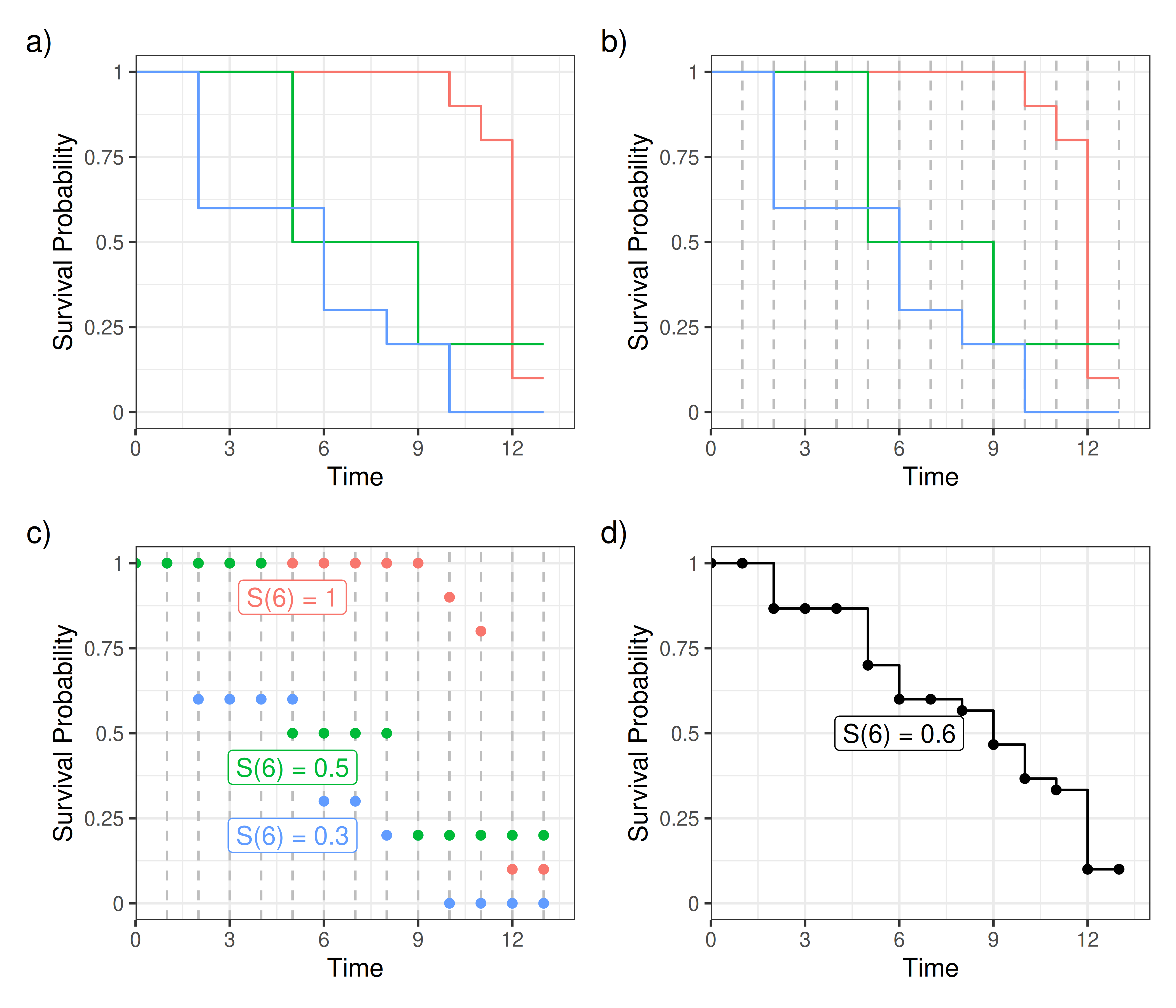
An important practical consideration is how to average survival probabilities across decision trees, as each individual non-parametric estimate may be defined on different event times. This is addressed by leveraging the fact that non-parametric estimators are step functions. For example, the Kaplan-Meier estimator is constant between event times and equal to the most recently observed survival probability, effectively allowing the estimator to make predictions at arbitrary time points as discussed in (Section 11.1). Figure 12.5 demonstrates the process for three decision trees, where panel (a) shows the estimates within three terminal nodes (red, green, blue). Each Kaplan-Meier estimator is evaluated at the union of observed event times across trees (panels b-c), and the resulting survival probabilities are averaged at each time point to obtain the bootstrapped survival estimate (12.3), shown in panel (d).
12.2.3 Competing risks
The RSF framework extends to competing risks (Section 4.2) in a natural way, replacing the single-event Kaplan-Meier and Nelson-Aalen estimators in the terminal nodes with the Aalen-Johansen CIF estimator (Section 4.2.2; Ishwaran et al. (2014)). Both the splitting rule and the terminal node estimator must be adapted to account for the presence of multiple event types.
12.2.3.1 Splitting rules
Splitting rules can be separated into cause-specific and composite splitting rules (Ishwaran et al. 2014). Cause-specific rules target a single cause \(q\) and are appropriate when the primary interest is in one particular cause. Composite rules aggregate information across all \(Q\) causes and are appropriate when the goal is to predict all cause-specific hazards or CIFs simultaneously. Composite rules produce a single splitting statistic by taking a variance-weighted sum of the per-cause statistics across all \(Q\) causes (Ishwaran et al. 2014).
Two common splitting rules are the generalized log-rank rule and Gray’s test. The generalized log-rank rule tests \(H_0: h_q^l = h_q^r\), where \(h_q\) is the hazard for cause \(q\), whereas Gray’s test tests \(H_0: F_q^l = F_q^r\), where \(F_q\) is the CIF for cause \(q\).
Generalized log-rank. The cause-\(q\) log-rank statistic treats competing events as censored, so that the risk set for cause \(q\) consists of all subjects still at risk for any event, with the number of subjects at risk denoted by \(n_{\tau}\). The observed cause-\(q\) events in \(\mathcal{A}^l\) at some \(\tau\) are:
\[ o^l_{q,{\tau}} = \sum_{i \in \mathcal{A}^l} \mathbb{I}(t_i = \tau,\, q_i = q), \]
where \(q_i\) is the observed cause for observation \(i\). The expected number of events under the null of equal cause-\(q\) hazards in both nodes is:
\[ e^l_{q,{\tau}} = o_{q,{\tau}}\frac{n^l_{\tau}}{n_{\tau}}, \tag{12.5}\]
where \(o_{q,{\tau}}\) and \(n_{\tau}\) are the corresponding totals over both nodes. The per-cause statistic for \(m\) ordered event times, \(t_{(k)}\), is:
\[ LR_q(\mathcal{A}^l) = \frac{\sum^m_{k=1} w_q({t_{(k)}})\,(o^l_{q,{t_{(k)}}} - e^l_{q,{t_{(k)}}})}{\sqrt{\sum^m_{k=1} w_q({t_{(k)}})^2\, v^l_{q,{t_{(k)}}}}}, \tag{12.6}\]
where \(v^l_{q,{t_{(k)}}}\) is the hypergeometric variance for cause \(q\) at \(t_{(k)}\), and \(w_q(t_{(k)}) > 0\) are time-dependent weights that can be used to up-weight differences at the beginning or end of follow-up (Harrington and Fleming 1982).
The composite log-rank statistic aggregates the per-cause statistics (12.6) across all \(Q\) causes:
\[ LR_{CR}(\mathcal{A}^l) = \frac{\sum_{q=1}^Q \hat{\sigma}_q^2 \, LR_q(\mathcal{A}^l)}{\sqrt{\sum_{q=1}^Q \hat{\sigma}_q^2}}, \qquad \hat{\sigma}_q^2 = \sum_k w_q({t_{(k)}})^2\, v^l_{q,{t_{(k)}}}; \]
Gray’s test. While the generalized log-rank rule detects variables that affect the cause-\(q\) hazard, Gray’s test (Gray 1988) instead tests \(H_0: F_q^l = F_q^r\), thereby selecting variables according to differences in the cumulative incidence of cause \(q\). As Gray’s test targets the CIF directly, it could be preferred when the CIF is the prediction of interest in the competing risks setting (Ishwaran et al. 2014).
Following Ishwaran et al. (2014), the splitting statistic is obtained by substituting an augmented risk set into (12.5) in place of \(n_{t_{(k)}}\). Motivated by the Fine-Gray subdistribution hazard framework (Section 11.2.3), the augmented risk set retains subjects who experienced a competing event before \(t_{(k)}\). In practice, this is implemented by adding subjects who experienced a competing event before \(t_{(k)}\) back into the risk set (Fine and Gray 1999):
\[ \tilde{n}_{q,t_{(k)}} = n_{t_{(k)}} + \sum_{j:\, t_{(j)} < t_{(k)}} \sum_{q' \neq q} d_{q',t_{(j)}}. \]
The observed cause-\(q\) events are unchanged:
\[ o^l_{q,t_{(k)}} = \sum_{i \in \mathcal{A}^l} \mathbb{I}(t_i = t_{(k)},\, q_i = q). \]
The expected count replaces \(n_{t_{(k)}}\) with \(\tilde{n}_{q,t_{(k)}}\) (and \(n^l_{t_{(k)}}\) with \(\tilde{n}^l_{q,t_{(k)}}\)) in (12.5):
\[ \tilde{e}^l_{q,t_{(k)}} = o_{q,t_{(k)}}\frac{\tilde{n}^l_{q,t_{(k)}}}{\tilde{n}_{q,t_{(k)}}}. \]
The per-cause Gray statistic is then:
\[ \widetilde{LR}_q(\mathcal{A}^l) = \frac{\sum_{k} w_q(t_{(k)})\,(o^l_{q,t_{(k)}} - \tilde{e}^l_{q,t_{(k)}})}{\sqrt{\sum_{k} w_q(t_{(k)})^2\,\tilde{v}^l_{q,t_{(k)}}}}, \]
where \(\tilde{v}^l_{q,t_{(k)}}\) is the hypergeometric variance (12.6) with \(\tilde{n}_{q,t_{(k)}}\) in place of \(n_{t_{(k)}}\).
Similarly to the cause-specific case, the composite Gray statistic is:
\[ \widetilde{LR}(\mathcal{A}^l) = \frac{\sum_{q=1}^Q \tilde{\sigma}_q^2 \, \widetilde{LR}_q(\mathcal{A}^l)}{\sqrt{\sum_{q=1}^Q \tilde{\sigma}_q^2}}, \qquad \tilde{\sigma}_q^2 = \sum_k w_q(t_{(k)})^2\,\tilde{v}^l_{q,t_{(k)}}. \]
12.2.3.2 Terminal node prediction
Within each terminal node \(\mathcal{A}_b(\mathbf{x}_*)\), the Aalen-Johansen estimator is used to estimate the CIF for each cause \(q \in \{1, \ldots, Q\}\).
Let \(t^*_{(1)} < \ldots < t^*_{(m)}\) be the ordered event times (of any cause) within \(\mathcal{A}_b(\mathbf{x}_*)\), and let \(d_{q,t^*_{(k)}}\) and \(n_{t^*_{(k)}}\) denote the number of cause-\(q\) events and the number at risk at \(t^*_{(k)}\), both computed from observations in \(\mathcal{A}_b(\mathbf{x}_*)\). The cause-specific discrete hazard (Section 4.2.2) within the node is \(\hat{h}^d_{q,b}(t^*_{(k)}) = d_{q,t^*_{(k)}} / n_{t^*_{(k)}}\), the all-cause survival in the node is then,
\[ \hat{S}_b(\tau \mid \mathbf{x}_*) = \prod_{k: t^*_{(k)} \leq \tau} \left(1 - \sum_{q=1}^Q \hat{h}^d_{q,b}(t^*_{(k)})\right), \]
and the CIF for cause \(q\) is the discrete Aalen-Johansen estimator,
\[ \hat{F}_{q,b}(\tau \mid \mathbf{x}_*) = \sum_{k: t^*_{(k)} \leq \tau} \hat{S}_b(t^*_{(k-1)} \mid \mathbf{x}_*) \hat{h}^d_{q,b}(t^*_{(k)}), \]
with \(t^*_{(0)} = 0\).
Finally, the bootstrapped CIF prediction is the weighted average of the per-tree Aalen-Johansen estimates:
\[ \hat{F}_{q,Boot}(\tau \mid \mathbf{x}_*) = \sum_{b=1}^B w_b\hat{F}_{q,b}(\tau \mid \mathbf{x}_*). \]
As with the bootstrapped Kaplan-Meier prediction (12.3), the ensemble CIF also represents a mixture of the per-tree distributions.
12.2.4 Relative risk predictions
The most common method to estimate the average relative risk appears to be a transformation from the Nelson-Aalen method (Ishwaran et al. 2008), which exploits results from counting processes to provide a measure of expected mortality (Hosmer Jr et al. 2011); the same result is used in the event frequency calibration measure discussed in Section 7.1.2. The logic is that the resulting estimation is proportional to the expected number of events in \(\mathcal{A}_b(\mathbf{x}_*)\) and it is natural to assume a terminal node with more expected events represents a higher risk group.
Given new data \(\mathbf{x}_*\) falling into terminal node \(\mathcal{A}_b(\mathbf{x}_*)\), the relative risk prediction is the sum of the predicted cumulative hazard \(\hat{H}_b(\cdot \mid \mathbf{x}_*)\) over the observed times in that node:
\[ \phi_b(\mathbf{x}_*) = \sum_{i \in \mathcal{A}_b(\mathbf{x}_*)} \hat{H}_b(t_i \mid \mathbf{x}_*). \]
The bootstrapped risk prediction is the weighted average over all trees:
\[ \phi_{Boot}(\mathbf{x}_*) = \sum_{b=1}^B w_b\, \phi_b(\mathbf{x}_*). \tag{12.7}\]
More complex methods have also been proposed using likelihood-based splitting rules while assuming a PH model form (Ishwaran et al. 2004; LeBlanc and Crowley 1992), but these do not appear to be in widespread usage.
A similar method follows in the competing risks setting using predicted CIFs (Ishwaran et al. 2014):
\[ \phi_{q;b}(\mathbf{x}_*) = \int^{\tau^*}_0 \hat{F}_{q;b}(\tau \mid \mathbf{x}_*) \ d\tau, \]
where \(\tau^*\) is suggested to be the end of the study period. \(\phi_{q;Boot}(\mathbf{x}_*)\) is computed as in (12.7).